Canonical Tracing Form

This example demonstrates tracing charged particles using the canonical Hamiltonian formulation in $(\mathbf{x},\mathbf{p})$ phase space coordinates, compared against the standard velocity formulation $(\mathbf{x},\mathbf{v})$.

Motivation: Why Canonical Coordinates?

In Hamiltonian mechanics, the motion of a charged particle in an electromagnetic field with scalar potential $\varphi (\mathbf{x},t)$ and vector potential $\mathbf{A}(\mathbf{x},t)$ is governed by the canonical Hamiltonian:

$$H(\mathbf{x},\mathbf{p},t)=\frac{1}{2m}(\mathbf{p}-q\mathbf{A}(\mathbf{x},t){)}^2+q\varphi (\mathbf{x},t)$$

in the non-relativistic regime, and:

$$H(\mathbf{x},\mathbf{p},t)=\sqrt{m^2{c}^4+c^2(\mathbf{p}-q\mathbf{A}(\mathbf{x},t){)}^2}+q\varphi (\mathbf{x},t)$$

in the relativistic regime.

While standard particle pushers (such as Boris) operate on velocity $(\mathbf{x},\mathbf{v})$ directly from $(\mathbf{E},\mathbf{B})$ fields, the canonical formulation offers two major benefits:

1. Exact Preservation of Noether Symmetries (Cyclic Momenta): If the system has a spatial symmetry (e.g. axisymmetry in tokamaks or translational invariance in 1D/2D models), the corresponding canonical momentum $p_k$ is strictly conserved to machine precision across all ODE solvers. In velocity coordinates, kinematic velocity $v_k$ continuously rotates, accumulating secular drift in the invariant.

2. Canonical Symplectic Integration: Standard symplectic integrators (such as ImplicitMidpoint) directly preserve the canonical 2-form $\omega =\sum d{x}_i\wedge d{p}_i$ and maintain bounded energy oscillations over long integration times.

using TestParticle
using OrdinaryDiffEq, OrdinaryDiffEqSDIRK
using StaticArrays
using LinearAlgebra: norm
using CairoMakie

PotentialField & Non-Relativistic Landau Gauge

In a uniform magnetic field $\mathbf{B}=(0,0,B_0)$, we choose the Landau gauge $\mathbf{A}=(0,B_{0}x,0)$. Because the Hamiltonian does not depend on $y$ (${\partial }_{y}H=0$), the canonical momentum $p_y=m{v}_y+q{A}_y$ is a strict invariant of motion.

q = 1.0
m = 1.0
B0 = 1.0
Ω = q * B0 / m
T_period = 2π / Ω

# Define the vector potential; ForwardDiff automatically computes ∇A
A_landau(x) = SA[0.0, B0 * x[1], 0.0]
pf = PotentialField(A_landau)
param_can = prepare(pf; q = q, m = m)

# Initial condition: particle starting at origin moving in x direction
x0 = SA[0.0, 0.0, 0.0]
v0 = SA[1.0, 0.0, 0.0]
u0_can = velocity_to_canonical(x0, v0, param_can; relativistic = false)

t_end = 20 * T_period
tspan = (0.0, t_end)
dt = T_period / 40

# Trace in canonical form using ImplicitMidpoint
prob_can = TraceCanonicalProblem(u0_can, tspan, param_can; relativistic = false)
sol_can = solve(prob_can, ImplicitMidpoint(); dt = dt, adaptive = false)

# Trace in velocity form using Boris
param_xv = prepare(ZeroField(), (x, t) -> SA[0.0, 0.0, B0]; q = q, m = m)
prob_xv = TraceProblem([x0..., v0...], tspan, param_xv)
sol_xv = TestParticle.solve(prob_xv, Boris(); dt);

Comparing Cyclic Momentum Conservation

In velocity coordinates, $p_y(t)=m{v}_y(t)+q{B}_{0}x(t)$. We compare the drift in $p_y$ relative to its initial value ($p_y(0)=0$).

ts_can = sol_can.t ./ T_period
py_can_err = [abs(u[5] - u0_can[5]) for u in sol_can.u]

ts_xv = sol_xv.t ./ T_period
py_xv_err = [abs(m * u[5] + q * B0 * u[1] - u0_can[5]) for u in sol_xv.u]

fig1 = Figure(size = (800, 450))
ax1 = Axis(
    fig1[1, 1],
    xlabel = "Gyrations (t / T)",
    ylabel = "|p_y(t) - p_y(0)|",
    yscale = log10,
    title = "Conservation of Cyclic Momentum (p_y) in Landau Gauge"
)
lines!(ax1, ts_xv, max.(py_xv_err, 1.0e-16), label = "Boris (x, v)", color = :crimson)
lines!(ax1, ts_can, max.(py_can_err, 1.0e-16), label = "ImplicitMidpoint (x, p)", color = :teal)
axislegend(ax1, position = :rt)
fig1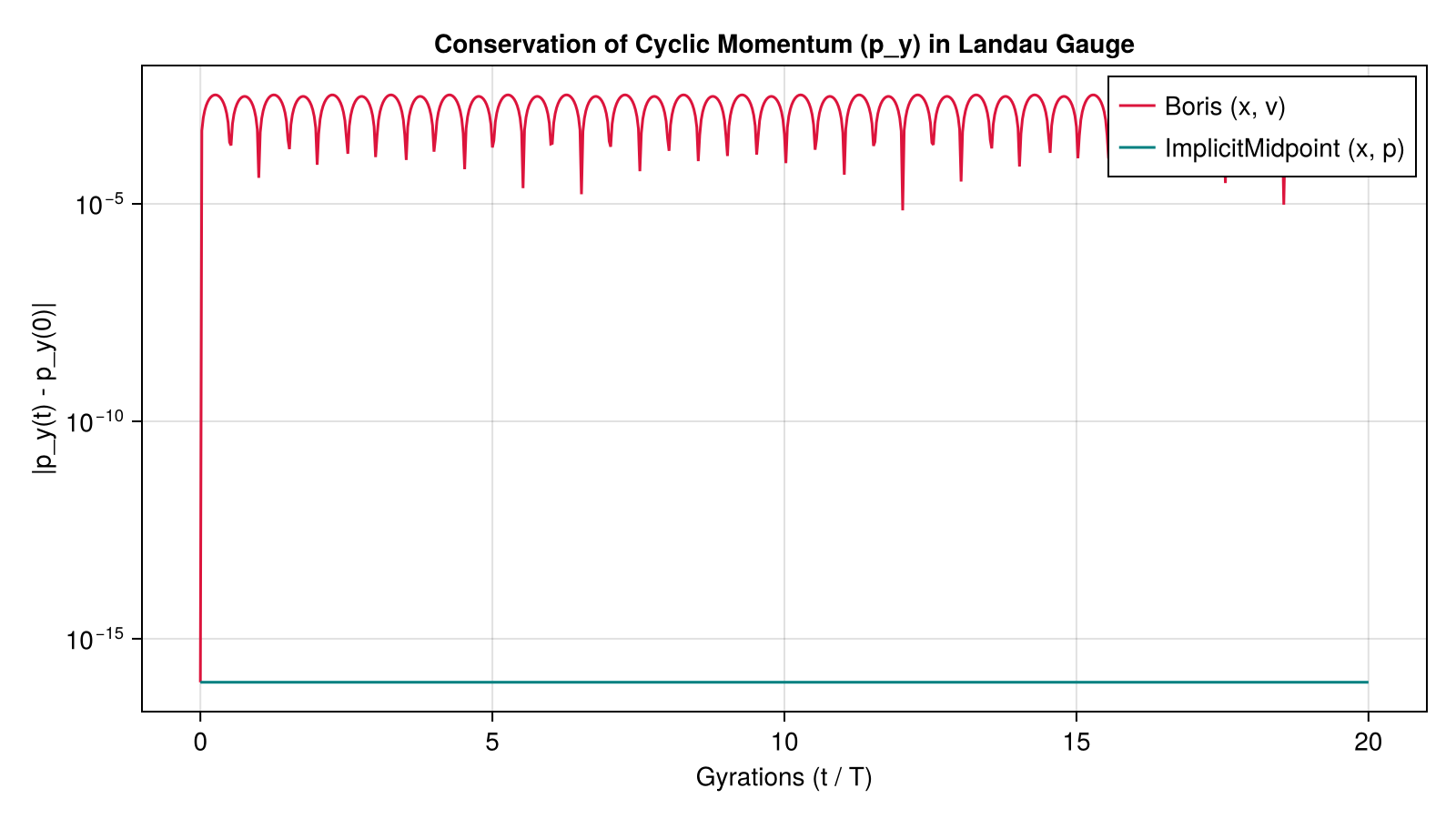

While Boris exhibits staggering phase oscillations of order $\sim {10}^{-3}$, the canonical solver preserves $p_y$ to exact machine zero across the entire simulation.

Relativistic Canonical Tracing

For relativistic dynamics ($v_0=0.6c$), we compare energy conservation and momentum tracking between the canonical formulation and velocity-space formulations.

c_val = 1.0
v0_rel = SA[0.6 * c_val, 0.0, 0.0]
param_can_rel = prepare(pf; q = q, m = m, c = c_val)
u0_can_rel = velocity_to_canonical(x0, v0_rel, param_can_rel; relativistic = true)

prob_can_rel = TraceCanonicalProblem(u0_can_rel, tspan, param_can_rel; relativistic = true)
sol_can_rel = solve(prob_can_rel, ImplicitMidpoint(); dt = dt, adaptive = false)

H0_rel = canonical_hamiltonian(sol_can_rel.u[1], param_can_rel; relativistic = true)
H_rel_err = [
    abs(canonical_hamiltonian(u, param_can_rel; relativistic = true) - H0_rel) / H0_rel
        for u in sol_can_rel.u
]

fig2 = Figure(size = (800, 450))
ax2 = Axis(
    fig2[1, 1],
    xlabel = "Gyrations (t / T)",
    ylabel = "Relative Energy Error |ΔH / H_0|",
    yscale = log10,
    title = "Relativistic Canonical Tracing: Bounded Symplectic Energy Error"
)
lines!(ax2, sol_can_rel.t ./ T_period, max.(H_rel_err, 1.0e-16), color = :midnightblue)
fig2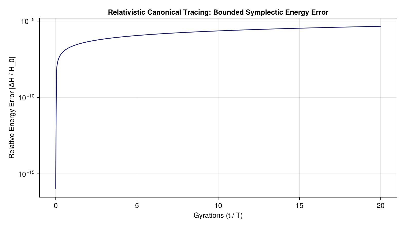

The Hamiltonian energy oscillates within a strictly bounded envelope without secular drift, confirming the structure-preserving property of the canonical symplectic integrator.