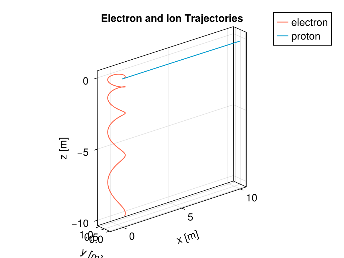
Proton and Electron

This example demonstrates tracing a single proton and electron motion under a uniform B field in real physical parameters. The E field is assumed to be zero such that there is no particle acceleration. Due to the fact that $m_{p} / m_{e} ≐ 1836$ , the proton gyro-radius is 1800 times larger than the electron, if they start with the same velocity as in this case. In more common cases we would compare electrons and protons with the same energy, and their gyro-radii differ by a factor of $\sqrt{m_{p} / m_{e}} \sim 40$ .

julia

using TestParticle, OrdinaryDiffEqVerner
using CairoMakie

### Initialize grid and field
x = range(-10, 10, length = 15)
y = range(-10, 10, length = 20)
z = range(-10, 10, length = 25)

B = fill(0.0, 3, length(x), length(y), length(z)) # [T]
E = fill(0.0, 3, length(x), length(y), length(z)) # [V/m]
B[3, :, :, :] .= 1e-11
E[3, :, :, :] .= 5e-13

### Initialize particles
stateinit = let
   x0 = [0.0, 0.0, 0.0] # initial position, [m]
   u0 = [1.0, 0.0, 0.0] # initial velocity, [m/s]
   [x0..., u0...]
end
param_electron = prepare(x, y, z, E, B, species = Electron)
tspan_electron = (0.0, 15.0)

param_proton = prepare(x, y, z, E, B, species = Proton)
tspan_proton = (0.0, 10.0)

### Solve for the trajectories
prob_e = ODEProblem(trace!, stateinit, tspan_electron, param_electron)
prob_p = ODEProblem(trace!, stateinit, tspan_proton, param_proton)

sol_e = solve(prob_e, Vern9())
sol_p = solve(prob_p, Vern9())

### Visualization
f = Figure(fontsize = 18)
ax = Axis3(f[1, 1],
   title = "Electron and Ion Trajectories",
   xlabel = "x [m]",
   ylabel = "y [m]",
   zlabel = "z [m]",
   aspect = :data
)
plot!(sol_e, idxs = (1, 2, 3), color = :tomato, label = "electron")
plot!(sol_p, idxs = (1, 2, 3), color = :deepskyblue3, label = "proton")

axislegend()

Proton and Electron ​

Proton and Electron