Dimensionless Units and Normalization

This example shows how to trace charged particles in dimensionless units.

Tracing in dimensionless units is beneficial for many scenarios. For example, MHD simulations do not have intrinsic scales. Therefore, we can do dimensionless particle tracing in MHD fields, and then convert to any scale we would like.

Normalization

After normalization, $q=1,B=1,m=1$ so that the gyroradius $r_L=m{v}_{\perp }/qB=v_{\perp }$. All the quantities are given in dimensionless units: if the magnetic field is homogeneous and the initial perpendicular velocity $v_{\perp 0}^{\prime }$ is 4, then the gyroradius is 4. To convert them to the original units, $v_{\perp }=v_{\perp }^{\prime }\ast U_0$ and $r_L=r_L^{\prime }\ast l_0=4\ast l_0$.

The Lorentz equation in SI units is written as

$$\frac{\mathrm{d}\mathbf{v}}{\mathrm{d}t}=\frac{q}{m}(\mathbf{v}\times \mathbf{B}+\mathbf{E})$$

It can be normalized to

$$\frac{\mathrm{d}{\mathbf{v}}^{\prime }}{\mathrm{d}{t}^{\prime }}={\mathbf{v}}^{\prime }\times {\mathbf{B}}^{\prime }+{\mathbf{E}}^{\prime }$$

with the following transformation

$$\begin{array}{rl}\mathbf{v}& ={\mathbf{v}}^{\prime }{V}_0\\ t& =t^{\prime }{t}_0=t^{\prime }{\mathrm{\Omega }}^{-1}=t^{\prime }\frac{m}{q{B}_0}\\ \mathbf{B}& ={\mathbf{B}}^{\prime }{B}_0\\ \mathbf{E}& ={\mathbf{E}}^{\prime }{E}_0={\mathbf{E}}^{\prime }{V}_0{B}_0\end{array}$$

where all the coefficients with subscript 0 are expressed in SI units. All the variables with a prime are written in the dimensionless units.

Basic Tracing

Now let's demonstrate this with trace_normalized!.

using TestParticle, OrdinaryDiffEqVerner, StaticArrays
using TestParticle: qᵢ, mᵢ, c
using CairoMakie

# Number of cells for the field along each dimension
nx, ny, nz = 4, 6, 8
# Unit conversion factors between SI and dimensionless units
B₀ = 10e-9            # [T]
Ω = abs(qᵢ) * B₀ / mᵢ # [1/s]
t₀ = 1 / Ω            # [s]
U₀ = 1.0              # [m/s]
l₀ = U₀ * t₀          # [m]
E₀ = U₀*B₀            # [V/m]
# All quantities are in dimensionless units
x = range(-10, 10, length = nx) # [l₀]
y = range(-10, 10, length = ny) # [l₀]
z = range(-10, 10, length = nz) # [l₀]

B = fill(0.0, 3, nx, ny, nz) # [B₀]
B[3, :, :, :] .= 1.0
E = fill(0.0, 3, nx, ny, nz) # [E₀]

param = prepare(x, y, z, E, B; species = User)

# Initial condition
stateinit = let
   x0 = [0.0, 0.0, 0.0] # initial position [l₀]
   u0 = [4.0, 0.0, 0.0] # initial velocity [v₀]
   [x0..., u0...]
end
# Time span
tspan = (0.0, π) # half gyroperiod

prob = ODEProblem(trace_normalized!, stateinit, tspan, param)
sol = solve(prob, Vern9())

### Visualization
f = Figure(fontsize = 18)
ax = Axis(f[1, 1],
   title = "Proton trajectory",
   xlabel = "X",
   ylabel = "Y",
   limits = (-4.1, 4.1, -8.1, 0.1),
   aspect = DataAspect()
)

lines!(ax, sol, idxs = (1, 2))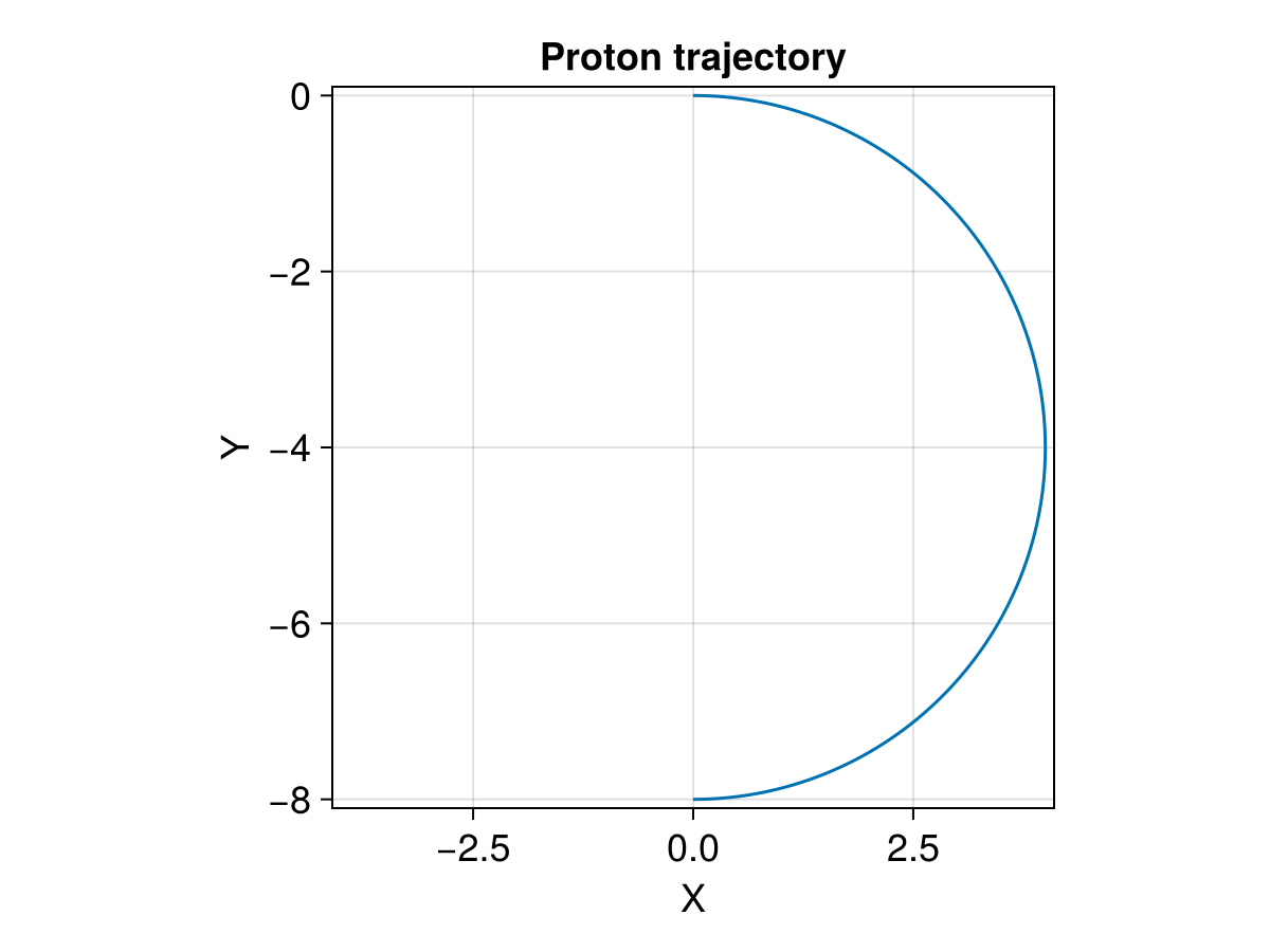

Relativistic Tracing

In the relativistic case,

• Velocity is normalized by speed of light c, $V=V^{\prime }c$;

• Magnetic field is normalized by the characteristic magnetic field, $B=B^{\prime }{B}_0$;

• Electric field is normalized by $E_0=c{B}_0$, $E=E^{\prime }{E}_0$;

• Location is normalized by the $L=c/{\mathrm{\Omega }}_0$, where ${\mathrm{\Omega }}_0=q{B}_0/m$, and

• Time is normalized by ${\mathrm{\Omega }}_0^{-1}$, $t=t^{\prime }\ast {\mathrm{\Omega }}_0^{-1}$.

In the small velocity scenario, it should behave similar to the non-relativistic case:

param = prepare(xu -> SA[0.0, 0.0, 0.0], xu -> SA[0.0, 0.0, 1.0]; species = User)
tspan = (0.0, π) # half period
stateinit = [0.0, 0.0, 0.0, 0.01, 0.0, 0.0]
prob = ODEProblem(trace_relativistic_normalized!, stateinit, tspan, param)
sol = solve(prob, Vern9())

### Visualization
f = Figure(fontsize = 18)
ax = Axis(f[1, 1],
   title = "Relativistic particle trajectory",
   xlabel = "X",
   ylabel = "Y",
   ##limits = (-0.6, 0.6, -1.1, 0.1),
   aspect = DataAspect()
)

lines!(ax, sol, idxs = (1, 2))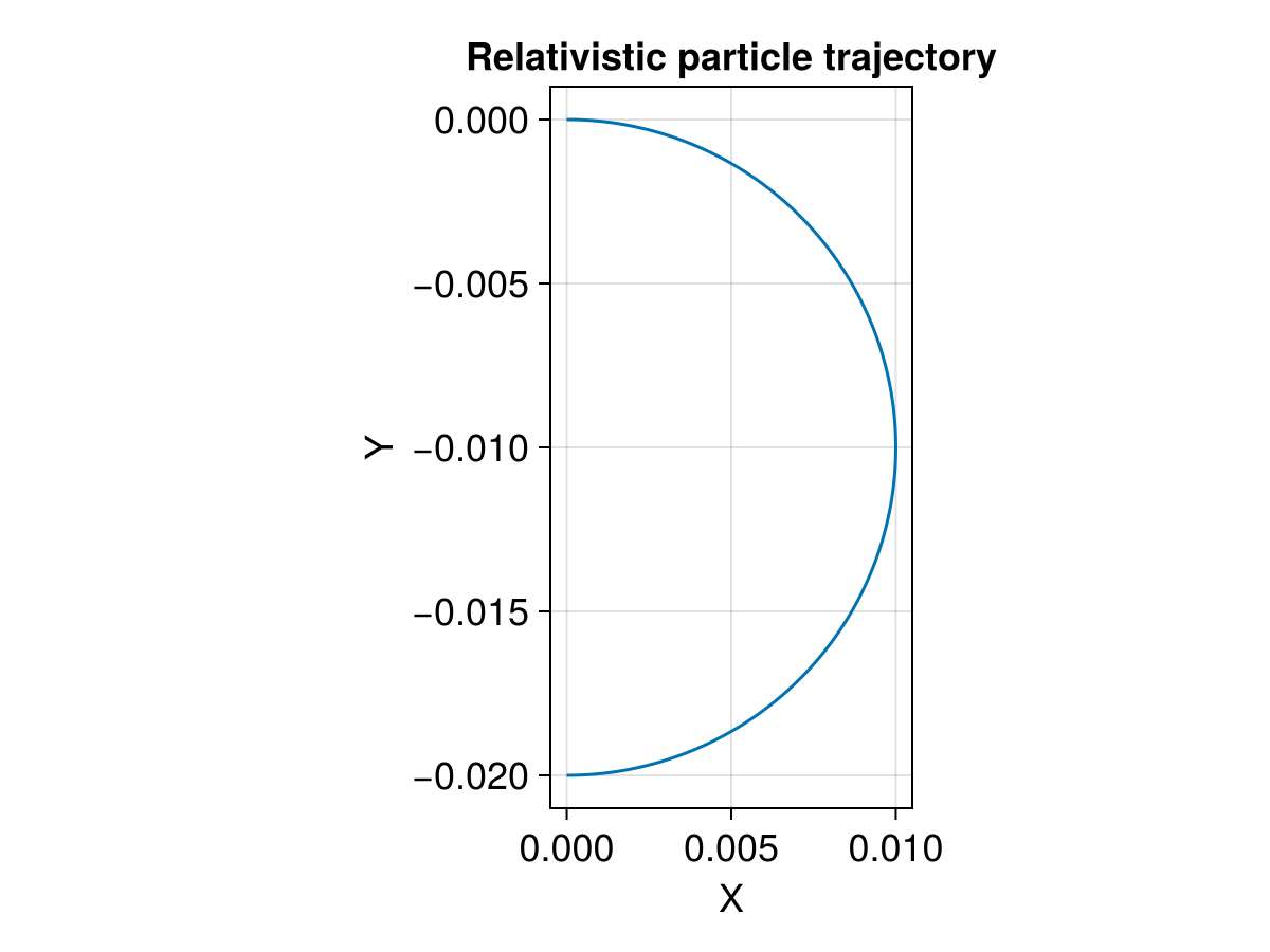

In the large velocity scenario, relativistic effect takes place:

param = prepare(xu -> SA[0.0, 0.0, 0.0], xu -> SA[0.0, 0.0, 1.0]; species = User)
tspan = (0.0, π) # half period
stateinit = [0.0, 0.0, 0.0, 0.9, 0.0, 0.0]
prob = ODEProblem(trace_relativistic_normalized!, stateinit, tspan, param)
sol = solve(prob, Vern9())

### Visualization
f = Figure(fontsize = 18)
ax = Axis(f[1, 1],
   title = "Relativistic particle trajectory",
   xlabel = "X",
   ylabel = "Y",
   aspect = DataAspect()
)

lines!(ax, sol, idxs = (1, 2))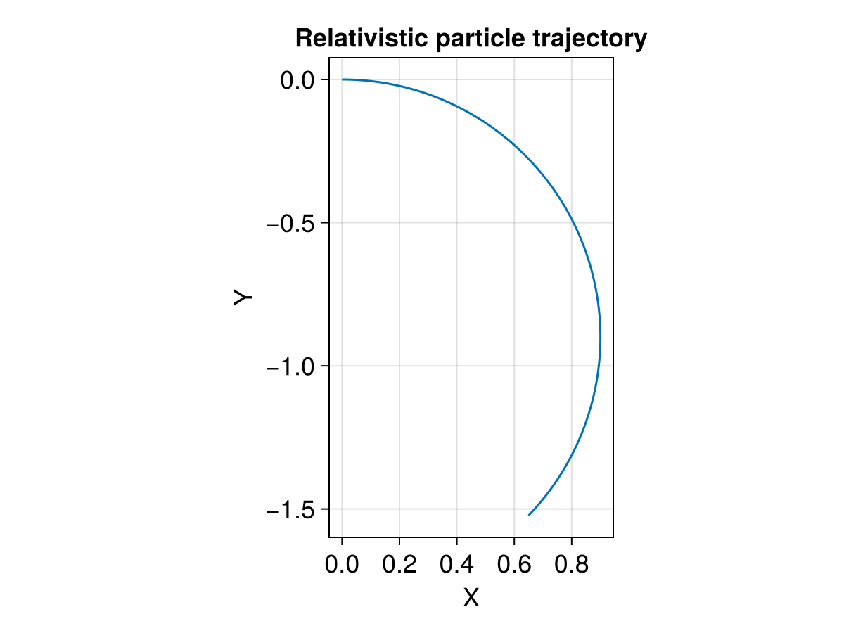

Dimensionless and Dimensional Tracing

We first solve the Lorentz equation in SI units, and then convert the quantities to normalized units and solve it again in dimensionless units.

# Unit conversion factors between SI and dimensionless units
B_dim = 1e-8             # [T]
U_dim = c                # [m/s]
E_dim = U_dim * B_dim    # [V/m]
Ω_dim = abs(qᵢ) * B_dim / mᵢ # [1/s]
t_dim = 1 / Ω_dim        # [s]
l_dim = U_dim * t_dim    # [m]
# Electric field magnitude in SI units
Emag_dim = 1e-8           # [V/m]
### Solving in SI units
B_field(x) = SA[0, 0, B_dim]
E_field(x) = SA[Emag_dim, 0.0, 0.0]

# Initial conditions
x0_dim = [0.0, 0.0, 0.0] # [m]
v0_dim = [0.0, 0.01c, 0.0] # [m/s]
stateinit1 = [x0_dim..., v0_dim...]
tspan1 = (0, 2π*t_dim) # [s]

param1 = prepare(E_field, B_field, species = Proton)
prob1 = ODEProblem(trace!, stateinit1, tspan1, param1)
sol1 = solve(prob1, Vern9(); reltol = 1e-4, abstol = 1e-6)

### Solving in dimensionless units
B_normalize(x) = SA[0, 0, B_dim / B_dim]
E_normalize(x) = SA[Emag_dim / E_dim, 0.0, 0.0]
# For full EM problems, the normalization of E and B should be done separately.
param2 = prepare(E_normalize, B_normalize; species = User)
# Scale initial conditions by the conversion factors
x0_norm = x0_dim ./ l_dim
v0_norm = v0_dim ./ U_dim
tspan2 = (0, 2π)
stateinit2 = [x0_norm..., v0_norm...]

prob2 = ODEProblem(trace_normalized!, stateinit2, tspan2, param2)
sol2 = solve(prob2, Vern9(); reltol = 1e-4, abstol = 1e-6)

### Visualization
f = Figure(fontsize = 18)
ax = Axis(f[1, 1],
   xlabel = "x [km]",
   ylabel = "y [km]",
   aspect = DataAspect()
)

lines!(ax, sol1, idxs = (1, 2))
# Interpolate dimensionless solutions and map back to SI units
xp, yp = let trange = range(tspan2..., length = 40)
   sol2.(trange, idxs = 1) .* l_dim, sol2.(trange, idxs = 2) .* l_dim
end
lines!(ax, xp, yp, linestyle = :dashdot, linewidth = 5, color = Makie.wong_colors()[2])
invL = inv(1e3)
scale!(ax.scene, invL, invL)

We see that the results are almost identical, with only floating point numerical errors. Tracing in dimensionless units usually allows larger timesteps, which leads to faster computation.

Tracing with Periodic Boundary

This example shows how to trace charged particles in dimensionless units and EM fields with periodic boundaries in a 2D spatial domain.

Now let's demonstrate this with trace_normalized!.

# Number of cells for the field along each dimension
nx, ny = 4, 6
# Unit conversion factors between SI and dimensionless units
B₀ = 10e-9            # [T]
Ω = abs(qᵢ) * B₀ / mᵢ # [1/s]
t₀ = 1 / Ω            # [s]
U₀ = 1.0              # [m/s]
l₀ = U₀ * t₀          # [m]
E₀ = U₀*B₀            # [V/m]

x = range(-10, 10, length = nx) # [l₀]
y = range(-10, 10, length = ny) # [l₀]

B = fill(0.0, 3, nx, ny) # [B₀]
B[3, :, :] .= 1.0

E_zero(x) = SA[0.0, 0.0, 0.0] # [E₀]

# If bc == 1, we set a NaN value outside the domain (default);
# If bc == 2, we set periodic boundary conditions.
param = prepare(x, y, E_zero, B; species = User, bc = 2);

Note that we set a radius of 10, so the trajectory extent from -20 to 0 in y, which is beyond the original y range.

# Initial conditions
stateinit = let
   x0 = [0.0, 0.0, 0.0] # initial position [l₀]
   u0 = [10.0, 0.0, 0.0] # initial velocity [v₀]
   [x0..., u0...]
end
# Time span
tspan = (0.0, 1.5π) # 3/4 gyroperiod

prob = ODEProblem(trace_normalized!, stateinit, tspan, param)
sol = solve(prob, Vern9());

Visualization

f = Figure(fontsize = 18)
ax = Axis(f[1, 1],
   title = "Proton trajectory",
   xlabel = "X",
   ylabel = "Y",
   limits = (-10.1, 10.1, -20.1, 0.1),
   aspect = DataAspect()
)

lines!(ax, sol, idxs = (1, 2))