---

title: Time-dependent B Field Tracing id: demo_coevolution date: 2026-01-28 author: "Hongyang Zhou" julia: 1.12 description: Tracing a particle in a time-dependent magnetic field. –-

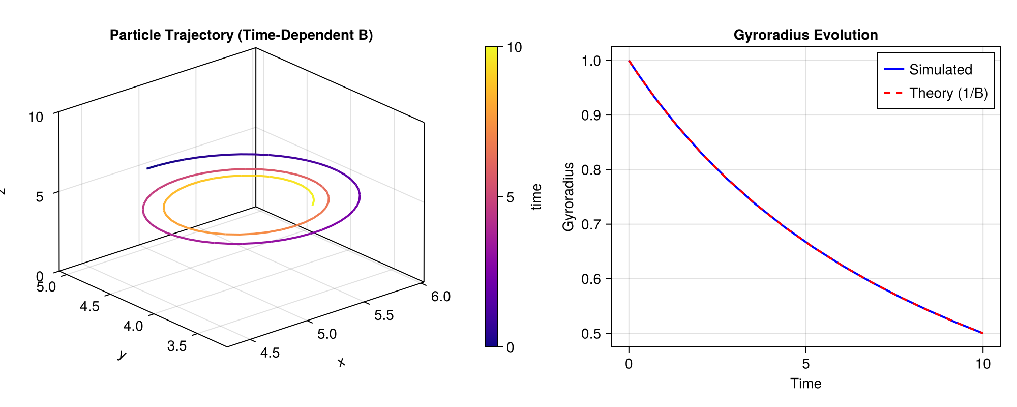
This example demonstrates how to trace a particle in a time-dependent numerical magnetic field. For analytical field, the time-dependency can be directly specified with time. For numerical field, the time-dependency can be specified with LazyTimeInterpolator that performs linear interpolation between time points. We will simulate a charged particle moving in a spatially uniform magnetic field that increases in magnitude over time. As the magnetic field strengthens, the particle's gyroradius is expected to shrink, demonstrating the co-evolution of the particle's orbit with the changing field. For simplicity, we neglect the electric field induced by the time-varying magnetic field, making particle's kinetic energy constant.

using TestParticle
import TestParticle as TP
using StaticArrays
using OrdinaryDiffEq
using LinearAlgebra
using CairoMakie

Define the Time-Dependent Field

We create a magnetic field $\mathbf{B}(t)=[0,0,B_z(t)]$ that is uniform in space but varies in time. The LazyTimeInterpolator allows us to define fields at specific time points and interpolate linearly between them.

times = [0.0, 10.0] # t=0 and t=10

# Spatial Grid (dummy, since the field is uniform)
gx = range(0.0, 10.0, length = 3)
gy = range(0.0, 10.0, length = 3)
gz = range(0.0, 10.0, length = 3)

# Filter function to generate the field at a given time index
function loader(i)
    # t=0 (i=1) -> B=1.0
    # t=10 (i=2) -> B=2.0
    val = (i == 1) ? 1.0 : 2.0

    B_data = fill(SVector{3}(0.0, 0.0, val), length(gx), length(gy), length(gz))

    return TP.getinterp(TP.CartesianGrid, B_data, gx, gy, gz)
end

loader (generic function with 1 method)

Create the time-dependent interpolator

itp_B = TP.LazyTimeInterpolator(times, loader)

# Define a zero Electric field
E_zero = TP.ZeroField();

Prepare Particle Tracing Parameters

We trace a dimensionless particle. We set q=1.0 and m=1.0. The prepare function sets up the equation of motion parameters.

param = prepare(gx, gy, gz, E_zero, itp_B; q = 1.0, m = 1.0);

Initial Conditions

We launch the particle with velocity purely perpendicular to the B field (in the x-direction). ${\mathbf{x}}_0=[5,5,5]$ (center of the domain) ${\mathbf{v}}_0=[1,0,0]$

x0 = SVector(5.0, 5.0, 5.0)
v0 = SVector(1.0, 0.0, 0.0)
stateinit = [x0..., v0...]
tspan = (0.0, 10.0);

Run the Simulation

We use trace_normalized! which is suitable for dimensionless or normalized tracing.

prob = ODEProblem(trace_normalized!, stateinit, tspan, param)
sol = solve(prob, Vern7());

Visualization

We visualize the results in two ways:

1. A 3D plot of the particle trajectory.

2. A time-series plot of the gyroradius $r_g=v_{\perp }/{\mathrm{\Omega }}_c$ to see it shrinking.

Calculate Gyroradius: $r_g=m{v}_{\perp }/(|q|B)$. Here m=1, q=1, v_perp = 1. $B(t)=1.0+0.1t$

f = Figure(size = (1000, 400))

# Plot 1: 3D Trajectory
nt = 101
ts = range(tspan..., length = nt)
x, y, z = sol(ts, idxs = 1).u, sol(ts, idxs = 2).u, sol(ts, idxs = 3).u
ax1 = Axis3(
    f[1, 1],
    title = "Particle Trajectory (Time-Dependent B)",
    xlabel = "x", ylabel = "y", zlabel = "z"
)
lines!(ax1, x, y, z, color = ts, colormap = :plasma, linewidth = 2)
Colorbar(f[1, 2], limits = (ts[1], ts[end]), colormap = :plasma, label = "time")

# Plot 2: Gyroradius Evolution
times_sim = sol.t
# Access state variables directly from solution
positions = [u[1:3] for u in sol.u]
velocities = [u[4:6] for u in sol.u]

Bs = [norm(itp_B(p, t)) for (p, t) in zip(positions, times_sim)]
r_sim = [norm(v[1:2]) / b for (v, b) in zip(velocities, Bs)]
r_theory = [1.0 / b for b in Bs]

ax2 = Axis(f[1, 3], title = "Gyroradius Evolution", xlabel = "Time", ylabel = "Gyroradius")
lines!(ax2, times_sim, r_sim; label = "Simulated", color = :blue, linewidth = 2)
lines!(
    ax2, times_sim, r_theory;
    label = "Theory (1/B)", color = :red, linestyle = :dash, linewidth = 2
)
axislegend(ax2)