Adiabatic Invariants Periods

This example demonstrates the three characteristic time scales (periods) associated with the three adiabatic invariants of charged particle motion in a dipole field:

1. Gyro-motion: The rapid rotation around the magnetic field lines.

2. Bounce motion: The oscillation between magnetic mirror points along the field line.

3. Drift motion: The slow azimuthal drift around the Earth.

We calculate these periods theoretically and verify them numerically using TestParticle.jl.

using TestParticle
using TestParticle: DipoleField, sph2cart, dipole_fieldline, Rₑ, mᵢ, qᵢ, c
using OrdinaryDiffEqVerner
using LinearAlgebra
using Statistics
using CairoMakie

Theoretical Estimates

For a proton in Earth's dipole field, we can estimate the three periods.

The magnetic field strength at the equator for L-shell $L$ is $B_{eq}=B_0/L^3$, where $B_0\approx 3.12\times {10}^{-5}$ T.

The gyro-period is ${\tau }_g=2\pi m/(qB)$.

The bounce period is approximately ${\tau }_b\approx \frac{4L{R}_E}{v}(1.30-0.56\sin {\alpha }_{eq})$.

The drift period is approximately ${\tau }_d\approx \frac{2\pi q{B}_0{R}_E^2}{3m{v}^{2}L(0.35+0.15\sin {\alpha }_{eq})}$.

# Parameters
L = 2.5             # L-shell
Ek_MeV = 10.0       # Kinetic energy in MeV
α_eq = deg2rad(30)  # Equatorial pitch angle
B₀ = 3.12e-5        # Dipole moment magnitude [T]

# Constants
Ek = Ek_MeV * 1e6 * 1.602e-19 # Energy in Joules
γ = 1 + Ek / (mᵢ * c^2)
v = c * sqrt(1 - 1 / γ^2)       # Velocity [m/s]
B_eq = B₀ / L^3               # Equatorial field [T]

# Theoretical periods
# 1. Gyro period (at equator)
Ω_eq = qᵢ * B_eq / (mᵢ * γ)
τ_g_theo = 2π / Ω_eq

# 2. Bounce period
τ_b_theo = 4 * L * Rₑ / v * (1.30 - 0.56 * sin(α_eq))

# 3. Drift period
# Relativistic correction factor for drift?
# Gradient drift v_d = ...
# Using approximation from literature (usually non-relativistic but we can adjust mass).
# Let's use the standard approximate formula.
τ_d_theo = 2π * qᵢ * B₀ * Rₑ^2 / (3 * mᵢ * γ * v^2 * L * (0.35 + 0.15 * sin(α_eq)))

println("Theoretical Gyro Period (Equator): $(round(τ_g_theo, digits=4)) s")
println("Theoretical Bounce Period:         $(round(τ_b_theo, digits=4)) s")
println("Theoretical Drift Period:          $(round(τ_d_theo, digits=4)) s")

Theoretical Gyro Period (Equator): 0.0332 s
Theoretical Bounce Period:         1.497 s
Theoretical Drift Period:          125.4908 s

Numerical Simulation

We simulate the particle trajectory using Vern9 solver.

# Initial condition
r₀ = sph2cart(L * Rₑ, π / 2, 0.0) # Equatorial plane, theta=pi/2, phi=0
vmag = v
# The dipole field at the equator points in the -z direction.
# To have a pitch angle of α_eq, we need the angle between v and -z to be α_eq.
# v_x = 0 (radial), v_y = v_perp (azimuthal), v_z = v_para (field-aligned)
v₀ = [0.0, vmag * sin(α_eq), -vmag * cos(α_eq)]

stateinit = [r₀..., v₀...]
param = prepare(DipoleField())
tspan = (0.0, 1.2 * τ_d_theo) # Run for slightly more than one drift period

prob = ODEProblem(trace!, stateinit, tspan, param)
sol = solve(prob, Vern9(); reltol = 1e-6, maxiters = 1e8);

Analysis and Visualization

# Extract positions
t = sol.t
x = @view sol[1, :]
y = @view sol[2, :]
z = @view sol[3, :];

1. Gyro Motion

Zoom in on a small segment at the beginning. Note that here we show the raw output; a more smoothed version can be shown via interpolation.

idx_zoom = 1:min(length(t), 50)
f1 = Figure(size = (800, 400))
ax1 = Axis(f1[1, 1], title = "Gyro Motion (Zoom)", xlabel = "x [Rₑ]",
   ylabel = "y [Rₑ]", aspect = DataAspect())
lines!(ax1, x[idx_zoom] ./ Rₑ, y[idx_zoom] ./ Rₑ)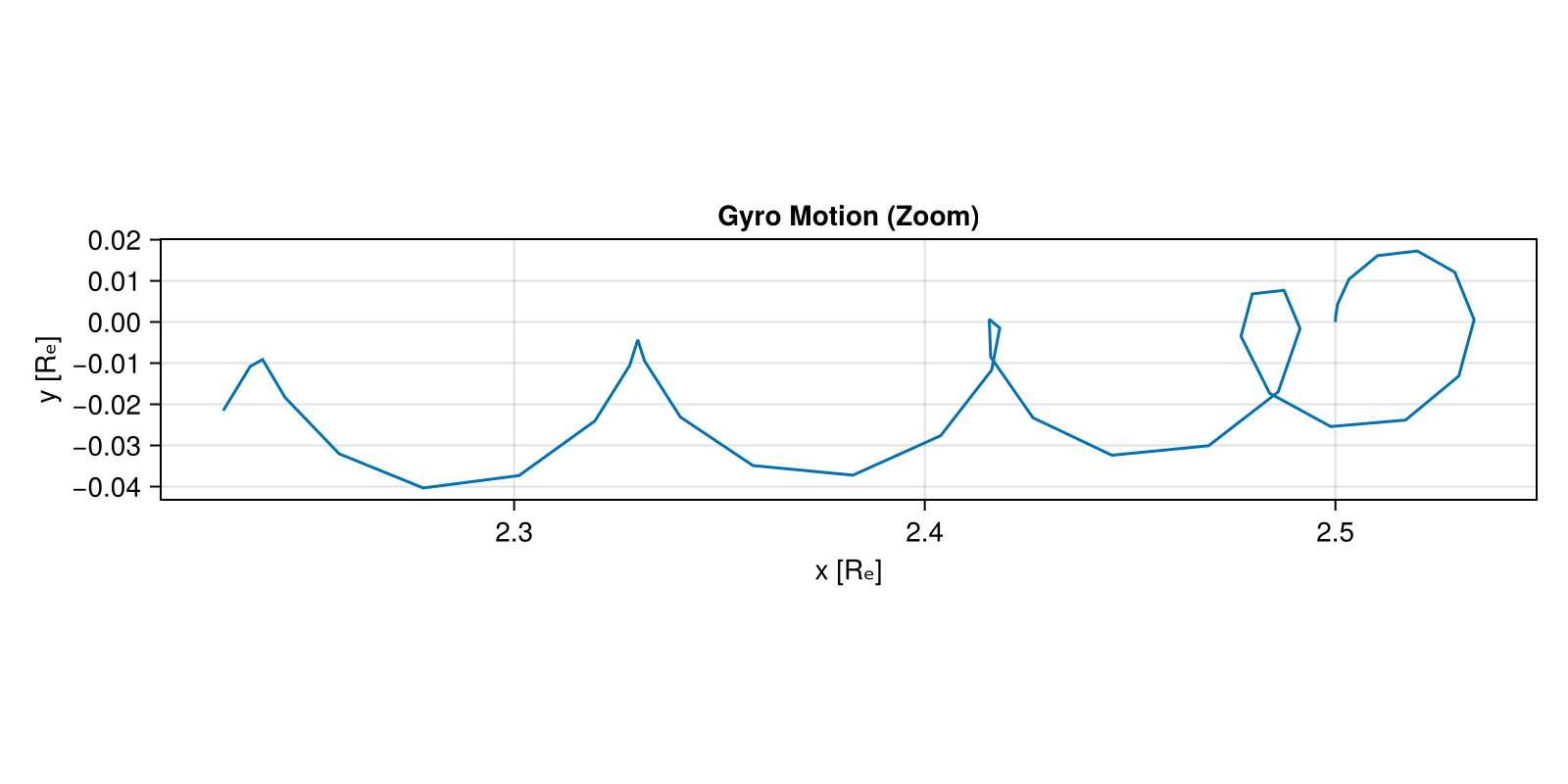

These does not look like full circles because the dipole field lines are curved, and as we move away from the equatorial plane, the perpendicular plane is no longer aligned with the X-Y plane.

2. Bounce Motion

Plot z-coordinate vs time to see bouncing.

f2 = Figure(size = (800, 400))
ax2 = Axis(f2[1, 1], title = "Bounce Motion", xlabel = "Time [s]", ylabel = "z [Rₑ]")
idx_bounce = t .< 10 * τ_b_theo
lines!(ax2, t[idx_bounce], z[idx_bounce] ./ Rₑ)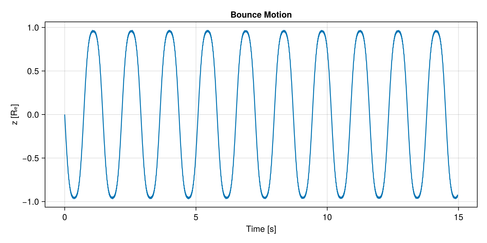

Calculate Bounce Period from z-crossings Find indices where z crosses 0 (approx).

signs = sign.(z)
crossings = findall(diff(signs) .!= 0)
if length(crossings) > 2
   t_cross = t[crossings]
   # Time between every second crossing is one period.
   τ_b_sim = mean(diff(t_cross)[1:2:(end - 1)]) * 2
   println("Simulated Bounce Period: $τ_b_sim s")
else
   println("Not enough bounces to estimate period.")
   τ_b_sim = NaN
end

Simulated Bounce Period: 1.4511602650005442 s

3. Drift Motion

# Plot x-y trajectory.
f3 = Figure(size = (600, 600))
ax3 = Axis(f3[1, 1], title = "Drift Motion (Azimuthal)",
   xlabel = "x [Rₑ]", ylabel = "y [Rₑ]", aspect = DataAspect())
lines!(ax3, x ./ Rₑ, y ./ Rₑ)
# Draw Earth
theta = LinRange(0, 2π, 100)
lines!(ax3, cos.(theta), sin.(theta), color = :black, linestyle = :dash)

Calculate Drift Period

# Calculate azimuthal angle phi, unwrap phi
phi_unwrap = let offset = 0.0
   phi = atan.(y, x)
   phi_unwrap = copy(phi)
   for i in eachindex(phi)[2:end]
      dphi = phi[i] - phi[i - 1]
      if dphi > π
         offset -= 2π
      elseif dphi < -π
         offset += 2π
      end
      phi_unwrap[i] += offset
   end
   phi_unwrap
end

# Fit line to phi vs t
# Slope is drift frequency.
slope = (phi_unwrap[end] - phi_unwrap[1]) / (t[end] - t[1])
τ_d_sim = abs(2π / slope)
println("Simulated Drift Period: $τ_d_sim s")

Simulated Drift Period: 122.51147888126152 s

Comparison table

Period	Theoretical	Simulated
Gyro	0.0332	N/A (varies)
Bounce	1.497	1.4512
Drift	125.4908	122.5115