Boris Method

This example demonstrates a single electron motion under a uniform B field. The E field is assumed to be zero such that there is no particle acceleration. We use the Boris method for phase space conservation under a fixed time step. This is compared against other ODE general algorithms for performance and accuracy.

using TestParticle, OrdinaryDiffEq, StaticArrays
using TestParticle: qᵢ, mᵢ
import TestParticle as TP
using CairoMakie

function plot_trajectory(
      sol_boris, sol1, sol2, sol_boris_2 = nothing, sol_boris_4 = nothing; alpha = 0.5)
   f = Figure(size = (700, 600), fontsize = 18)
   ax = Axis(f[1, 1], aspect = 1, limits = (-3, 1, -2, 2),
      xlabel = "X",
      ylabel = "Y")
   idxs = (1, 2)
   lines!(ax, sol1; idxs, color = (Makie.wong_colors()[1], alpha),
      linewidth = 2, linestyle = :dashdot, label = "Tsit5 fixed")
   lines!(ax, sol2; idxs, color = (Makie.wong_colors()[2], alpha), linewidth = 2,
      linestyle = :dashdot, label = "Tsit5 adaptive")
   lines!(ax, sol_boris; idxs, color = (Makie.wong_colors()[3], alpha),
      linewidth = 2, label = "Boris n=1")
   if !isnothing(sol_boris_2)
      lines!(ax, sol_boris_2; idxs, color = (Makie.wong_colors()[4], alpha),
         linewidth = 2, label = "Boris n=2")
   end
   if !isnothing(sol_boris_4)
      lines!(ax, sol_boris_4; idxs, color = (Makie.wong_colors()[5], alpha),
         linewidth = 2, label = "Boris n=4")
   end

   scale!(ax.scene, invrL, invrL)

   axislegend(position = :rt, framevisible = false)

   f
end

const Bmag = 0.01
uniform_B(x) = SA[0.0, 0.0, Bmag]
zero_E = TP.ZeroField()

x0 = [0.0, 0.0, 0.0]
v0 = [0.0, 1e5, 0.0]
stateinit = [x0..., v0...]
# (q2m, m, E, B, F)
param = prepare(zero_E, uniform_B, species = Electron)
q2m = TP.get_q2m(param)

# Reference parameters
const tperiod = 2π / (abs(q2m) *
                 sqrt(sum(x -> x^2, TP.get_BField(param)([0.0, 0.0, 0.0], 0.0))))
const rL = sqrt(v0[1]^2 + v0[2]^2 + v0[3]^2) / (abs(q2m) * Bmag)
const invrL = 1 / rL;

Multistep Boris Comparison

We first trace the particle for one period with a discrete time step of a quarter period.

tspan = (0.0, tperiod)
dt = tperiod / 4

prob = TraceProblem(stateinit, tspan, param)

sol_boris = TP.solve(prob; dt)[1];
sol_boris_2 = TP.solve(prob; dt, n = 2)[1];
sol_boris_4 = TP.solve(prob; dt, n = 4)[1];

Let's compare against the default ODE solver Tsit5 from DifferentialEquations.jl, in both fixed time step mode and adaptive mode:

prob = ODEProblem(trace!, stateinit, tspan, param)
sol1 = solve(prob, Tsit5(); adaptive = false, dt, dense = false, saveat = dt);
sol2 = solve(prob, Tsit5());

Visualization

f = plot_trajectory(sol_boris, sol1, sol2, sol_boris_2, sol_boris_4; alpha = 1)

It is clear that the Boris method comes with larger phase errors ($\mathcal{O}(\mathrm{\Delta }{t}^2)$) compared with Tsit5. See Phase Error Analysis for more details. The phase error gets smaller using a smaller dt:

dt = tperiod / 8

prob = TraceProblem(stateinit, tspan, param)

sol_boris = TP.solve(prob; dt)[1];
sol_boris_2 = TP.solve(prob; dt, n = 2)[1];
sol_boris_4 = TP.solve(prob; dt, n = 4)[1];

prob = ODEProblem(trace!, stateinit, tspan, param)
sol1 = solve(prob, Tsit5(); adaptive = false, dt, dense = false, saveat = dt);

Visualization

f = plot_trajectory(sol_boris, sol1, sol2, sol_boris_2, sol_boris_4; alpha = 1)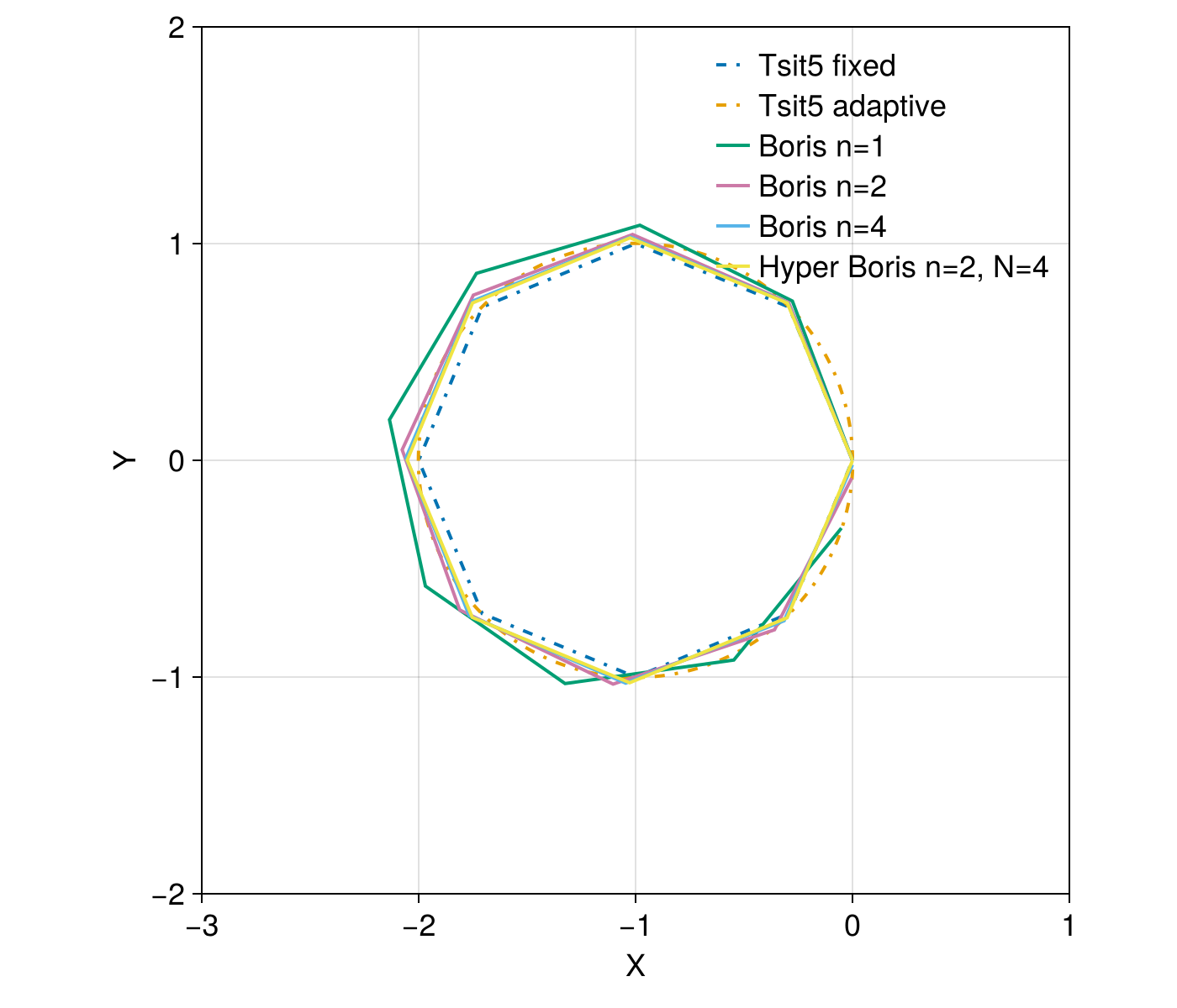

Energy Conservation

The Boris pusher shines when we do long time tracing, which is fast and conserves energy:

tspan = (0.0, 200 * tperiod)
dt = tperiod / 12

prob_boris = TraceProblem(stateinit, tspan, param)
prob = ODEProblem(trace!, stateinit, tspan, param)

sol_boris = TP.solve(prob_boris; dt, savestepinterval = 36)[1];
sol_boris_2 = TP.solve(prob_boris; dt, savestepinterval = 36, n = 2)[1];
sol_boris_4 = TP.solve(prob_boris; dt, savestepinterval = 36, n = 4)[1];
sol1 = solve(prob, Tsit5(); adaptive = false, dt, dense = false, saveat = dt);
sol2 = solve(prob, Tsit5());
sol3 = solve(prob, Vern7());
sol4 = solve(prob, Vern9());

Visualization

f = plot_trajectory(sol_boris, sol1, sol2)

Fixed time step Tsit5() is ok, but adaptive Tsit5() is pretty bad for long time evolutions. The change in radius indicates change in energy, which is known as numerical heating.

E_kin(vx, vy, vz) = 1 // 2 * (vx^2 + vy^2 + vz^2)
f = Figure(size = (800, 400), fontsize = 18)
ax = Axis(f[1, 1],
   xlabel = "time [period]",
   ylabel = "Normalized Kinetic Energy")

sols_to_plot = [
   (sol_boris, "Boris n=1"),
   (sol_boris_2, "Boris n=2"),
   (sol_boris_4, "Boris n=4"),
   (sol1, "Tsit5 fixed"),
   (sol2, "Tsit5 adaptive"),
   (sol3, "Vern7 adaptive"),
   (sol4, "Vern9 adaptive")
]

for (sol, label) in sols_to_plot
   energy = map(x -> E_kin(x[4:6]...), sol.u)
   lines!(ax, sol.t ./ tperiod, energy ./ energy[1], label = label, linewidth = 2)
end

axislegend(ax, position = :lt)

Advanced Boris Tracing

This section shows how to trace charged particles using the Boris method in dimensionless units with additionally boundary check. If the particles travel out of the domain specified by the field, the tracing will stop. Check Demo: Dimensionless Units for explaining the unit conversion.

"""
Set initial states.
"""
function prob_func(prob, i, repeat)
   prob = @views remake(prob; u0 = [prob.u0[1:3]..., 10.0 - i * 2.0, prob.u0[5:6]...])
end

isoutofdomain(xv, p, t) = isnan(xv[1])

# Number of cells for the field along each dimension
nx, ny = 4, 6
# Unit conversion factors between SI and dimensionless units
B₀ = 10e-9            # [T]
Ω = abs(qᵢ) * B₀ / mᵢ # [1/s]
t₀ = 1 / Ω            # [s]
U₀ = 1.0              # [m/s]
l₀ = U₀ * t₀          # [m]
E₀ = U₀ * B₀            # [V/m]

x = range(0, 11, length = nx) # [l₀]
y = range(-21, 0, length = ny) # [l₀]

B = fill(0.0, 3, nx, ny) # [B₀]
B[3, :, :] .= 1.0

E_field = TP.ZeroField() # [E₀]

# If bc == 1, we set a NaN value outside the domain (default);
# If bc == 2, we set periodic boundary conditions.
param = prepare(x, y, E_field, B; m = 1, q = 1, bc = 1)

(1.0, 1, TestParticle.ZeroField(), Field with interpolation support
Time-dependent: false
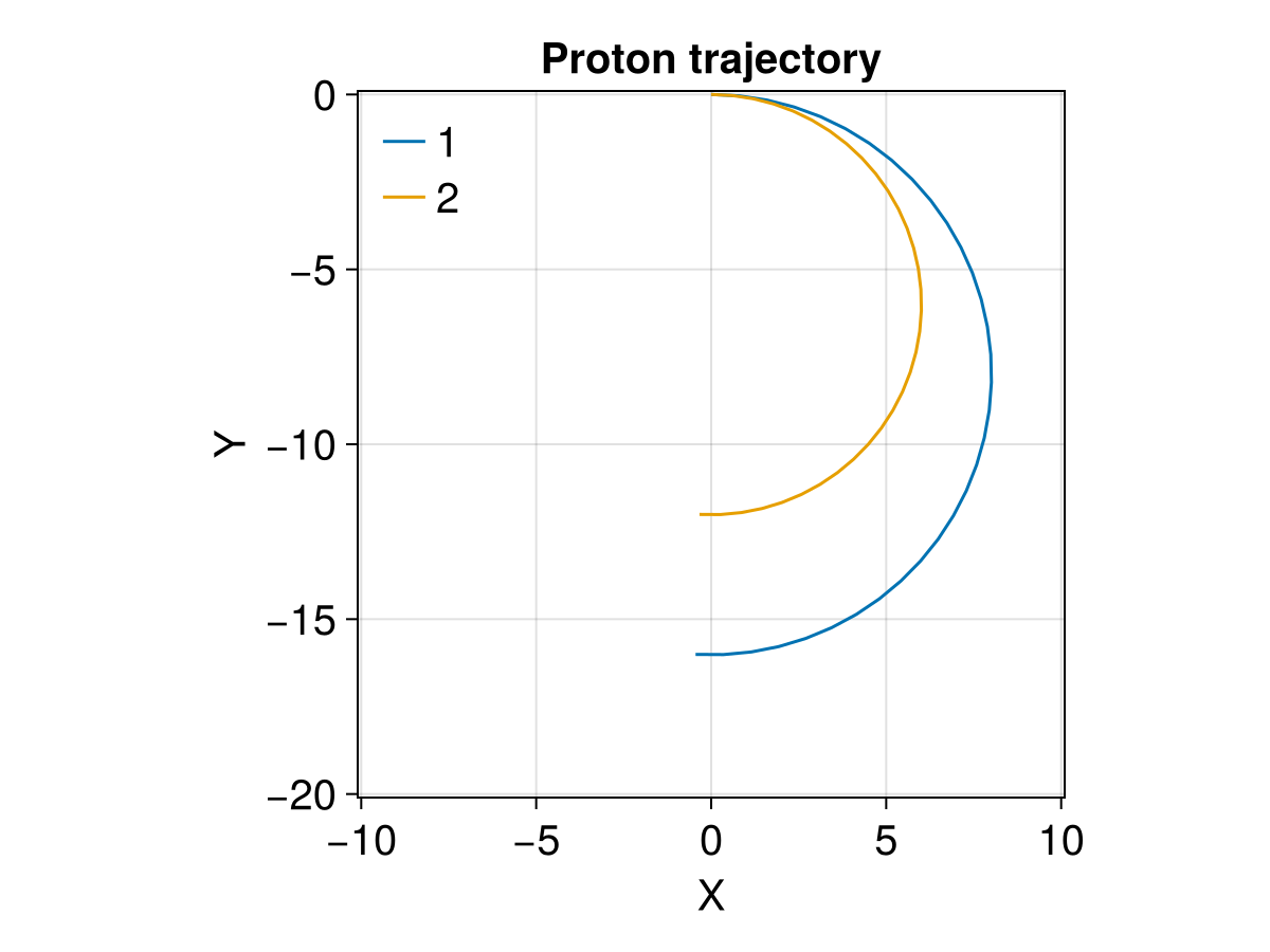
, TestParticle.ZeroField())

Note that we set a radius of 10 - 2i, where i is the index of the particle. The trajectory domain extends from -20 to 0 in y, and -10 to 10 in x. After half a cycle, the particle will move into the region where is field is not defined. The tracing will stop with the final step being all NaNs.

# Initial conditions to be modified in `prob_func`
x0 = [0.0, 0.0, 0.0] # initial position [l₀]
u0 = [0.0, 0.0, 0.0] # initial velocity [v₀], will be overwritten in prob_func
stateinit = [x0..., u0...]
tspan = (0.0, 1.5π) # 3/4 gyroperiod

dt = 0.1
savestepinterval = 1
trajectories = 2
prob = TraceProblem(stateinit, tspan, param; prob_func)

sols = TestParticle.solve(prob; dt, savestepinterval, isoutofdomain, trajectories)

f = Figure(fontsize = 18)
ax = Axis(f[1, 1],
   title = "Proton trajectory",
   xlabel = "X",
   ylabel = "Y",
   limits = (-10.1, 10.1, -20.1, 0.1),
   aspect = DataAspect()
)

for i in eachindex(sols)
   lines!(ax, sols[i]; idxs = (1, 2), label = string(i), color = Makie.wong_colors()[i])
end

axislegend(position = :lt, framevisible = false)