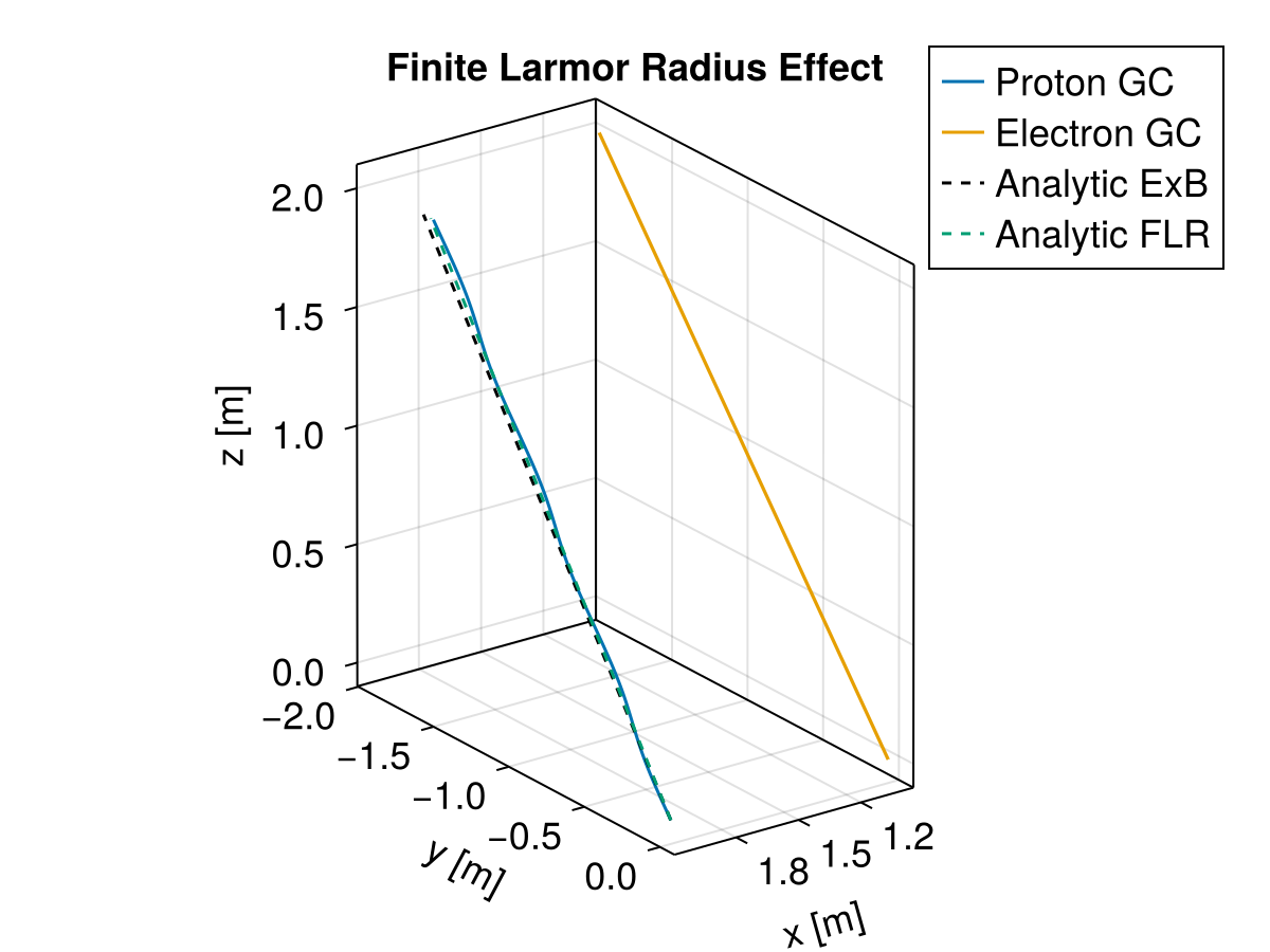
Finite-Larmor-Radius Effect

The general FLR effect refers to the correction terms introduced when considering the field difference at the particle location and the guiding center location. More theoretical details can be found in Non-uniform E Field.

using TestParticle, OrdinaryDiffEqVerner, StaticArrays
using LinearAlgebra: ×, ⋅, norm, normalize
using Tensors: laplace
import Tensors: Vec as Vec3
using CairoMakie

uniform_B(x) = SA[0, 0, 1e-8]

nonuniform_E(x) = SA[1e-9 * cos(0.3 * x[1]), 0, 0]

# Initial condition
stateinit = let x0 = [1.0, 0, 0], v0 = [0.0, 1.0, 0.1]
   [x0..., v0...]
end
# Time span
tspan = (0, 20)

# Proton
param_p = prepare(nonuniform_E, uniform_B, species = Proton)
prob_p = ODEProblem(trace!, stateinit, tspan, param_p)
sol_p = solve(prob_p, Vern9())

# Electron
param_e = prepare(nonuniform_E, uniform_B, species = Electron)
prob_e = ODEProblem(trace!, stateinit, tspan, param_e)
sol_e = solve(prob_e, Vern9())

# Analytic Drift (ExB + v_par)
# We use sol_p to provide v_par, but since B is uniform, ExB drift is independent of species/velocity.
# trace_gc_exb! calculates the guiding center drift without FLR corrections.
gc_p = param_p |> get_gc_func
gc_x0_p = gc_p(stateinit) |> Vector
prob_exb = ODEProblem(trace_gc_exb!, gc_x0_p, tspan, (param_p..., sol_p))
sol_exb = solve(prob_exb, Vern7())

# Analytic Drift with FLR
# Using Proton parameters and solution to calculate Larmor radius for FLR correction.
prob_flr = ODEProblem(trace_gc_flr!, gc_x0_p, tspan, (param_p..., sol_p))
sol_flr = solve(prob_flr, Vern7(); save_idxs = [1, 2, 3])

# numeric result and analytic result
f = Figure(fontsize = 18)
ax = Axis3(f[1, 1],
   title = "Finite Larmor Radius Effect",
   xlabel = "x [m]",
   ylabel = "y [m]",
   zlabel = "z [m]",
   aspect = :data,
   azimuth = 0.3π
)

# Plot Proton Guiding Center
gc_plot_p(x, y, z, vx, vy, vz) = (gc_p(SA[x, y, z, vx, vy, vz])...,)
lines!(ax, sol_p, idxs = (gc_plot_p, 1, 2, 3, 4, 5, 6),
   label = "Proton GC", color = Makie.wong_colors()[1])

# Plot Electron Guiding Center
gc_e = param_e |> get_gc_func
gc_plot_e(x, y, z, vx, vy, vz) = (gc_e(SA[x, y, z, vx, vy, vz])...,)
lines!(ax, sol_e, idxs = (gc_plot_e, 1, 2, 3, 4, 5, 6),
   label = "Electron GC", color = Makie.wong_colors()[2])

# Plot Analytic ExB Drift
lines!(
   ax, sol_exb, idxs = (1, 2, 3), label = "Analytic ExB", linestyle = :dash, color = :black)

# Plot Analytic FLR Drift
lines!(ax, sol_flr, idxs = (1, 2, 3), label = "Analytic FLR",
   linestyle = :dash, color = Makie.wong_colors()[3])

axislegend(ax)