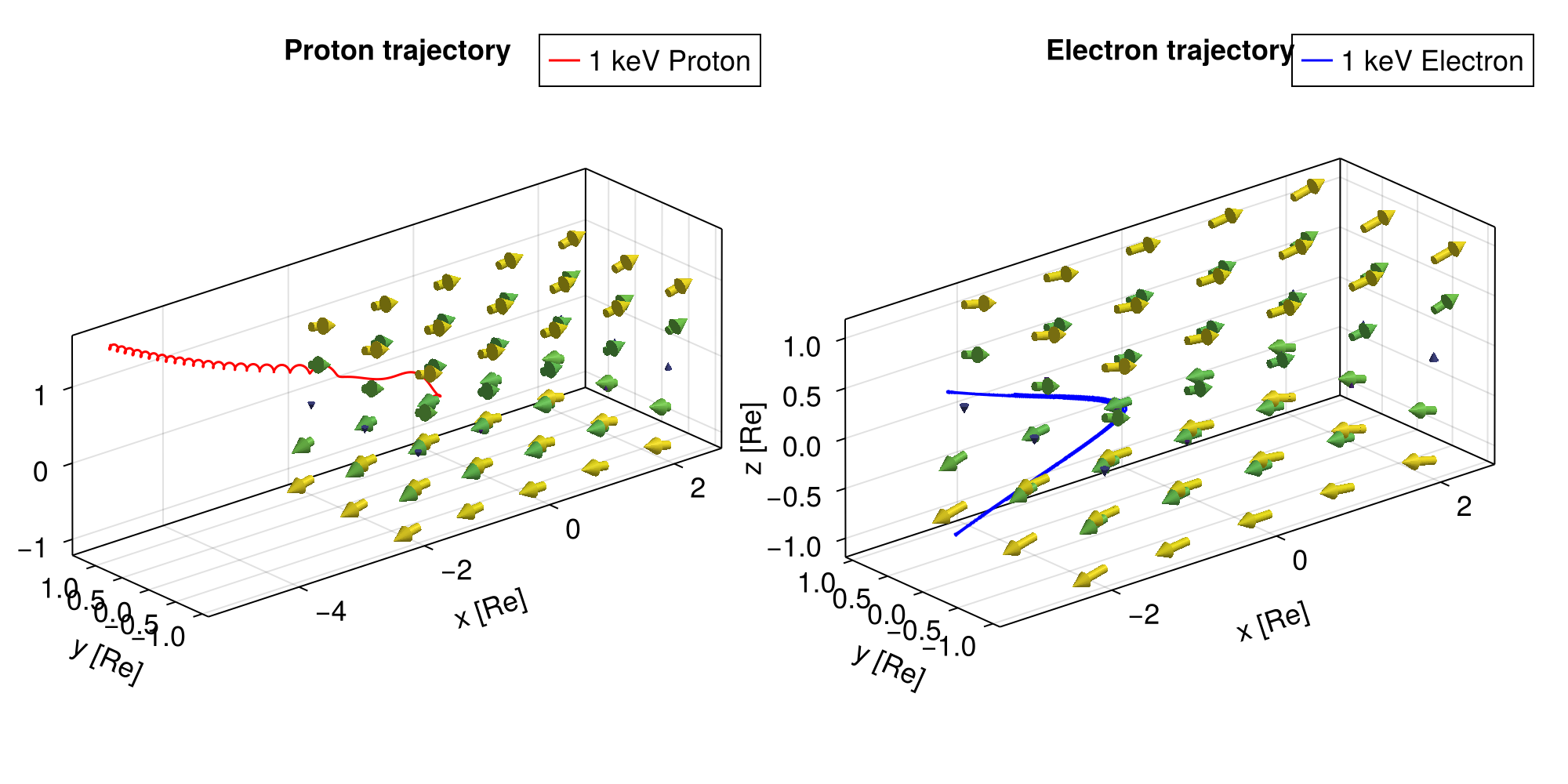
Reconnection X-line

This example traces protons and electrons near a magnetic reconnection X-line. The magnetic field is modeled as a Harris current sheet with a superposed X-type perturbation.

using TestParticle, OrdinaryDiffEq, StaticArrays
import TestParticle as TP
using TestParticle: Rₑ
using LinearAlgebra: norm
using CairoMakie

### Define the Field

# Parameters
const B₀ = 20e-9  # Asymptotic magnetic field [T]
const Bₙ = 1e-9   # Normal magnetic field gradient parameter [T]
const L = 0.5Rₑ   # Current sheet thickness [m]
const Eᵣ = 0.1e-3 # Reconnection electric field [V/m]

function getB(xu)
   x, y, z = xu[1], xu[2], xu[3]
   return SVector{3}(B₀ * tanh(z / L), 0.0, Bₙ * x / L)
end

getE(xu) = SVector{3}(0.0, Eᵣ, 0.0)

### Trace Particles

# Initialize proton
x0_p = [-1.0Rₑ, 0.0, 0.1Rₑ]
Ek_p = 1e3 # eV
v_p = TP.energy2velocity(Ek_p) # magnitude
v0_p = [v_p, 0.0, 0.0]

stateinit_p = [x0_p..., v0_p...]
param_p = prepare(getE, getB, species = TP.Proton)
tspan_p = (0.0, 100.0) # seconds

prob_p = ODEProblem(TP.trace!, stateinit_p, tspan_p, param_p)
sol_p = solve(prob_p, Vern9())

# Initialize electron
x0_e = [-1.0Rₑ, 0.0, 0.1Rₑ]
Ek_e = 1e3 # eV
v_e = TP.energy2velocity(Ek_e, m = TP.mₑ, q = TP.qₑ) # magnitude
v0_e = [v_e, 0.0, 0.0]

stateinit_e = [x0_e..., v0_e...]
param_e = prepare(getE, getB, species = TP.Electron)
tspan_e = (0.0, 15.0) # seconds, electron is much faster

prob_e = ODEProblem(TP.trace!, stateinit_e, tspan_e, param_e)
sol_e = solve(prob_e, Vern9())

### Visualization

f = Figure(size = (1000, 500), fontsize = 18)

function plot_trajectory!(fpos, sol, tspan, title, label, color)
   ax = Axis3(fpos,
      title = title,
      xlabel = "x [Re]",
      ylabel = "y [Re]",
      zlabel = "z [Re]",
      aspect = :data
   )

   n = 10000 # number of timepoints
   ts = range(tspan..., length = n)
   x = sol(ts, idxs = 1) ./ Rₑ |> Vector
   y = sol(ts, idxs = 2) ./ Rₑ |> Vector
   z = sol(ts, idxs = 3) ./ Rₑ |> Vector

   lines!(ax, x, y, z, label = label, color = color)
   axislegend(ax, backgroundcolor = :transparent)
   return ax
end

# Plot Proton
ax1 = plot_trajectory!(f[1, 1], sol_p, tspan_p, "Proton trajectory", "1 keV Proton", :red)

# Plot Electron
ax2 = plot_trajectory!(
   f[1, 2], sol_e, tspan_e, "Electron trajectory", "1 keV Electron", :blue)

# Add B field arrows to proton plot for context
function plot_B!(ax)
   xrange = range(-2, 2, length = 5)
   yrange = range(-1, 1, length = 3)
   zrange = range(-1, 1, length = 5)

   ps = [Point3f(x, y, z) for x in xrange for y in yrange for z in zrange]
   B = map(p -> Vec3f(getB(p .* Rₑ) ./ B₀), ps)
   Bmag = norm.(B)

   arrows!(ax, ps, B, fxaa = true, color = Bmag, lengthscale = 0.4, arrowsize = 0.05)
end

plot_B!(ax1)
plot_B!(ax2)