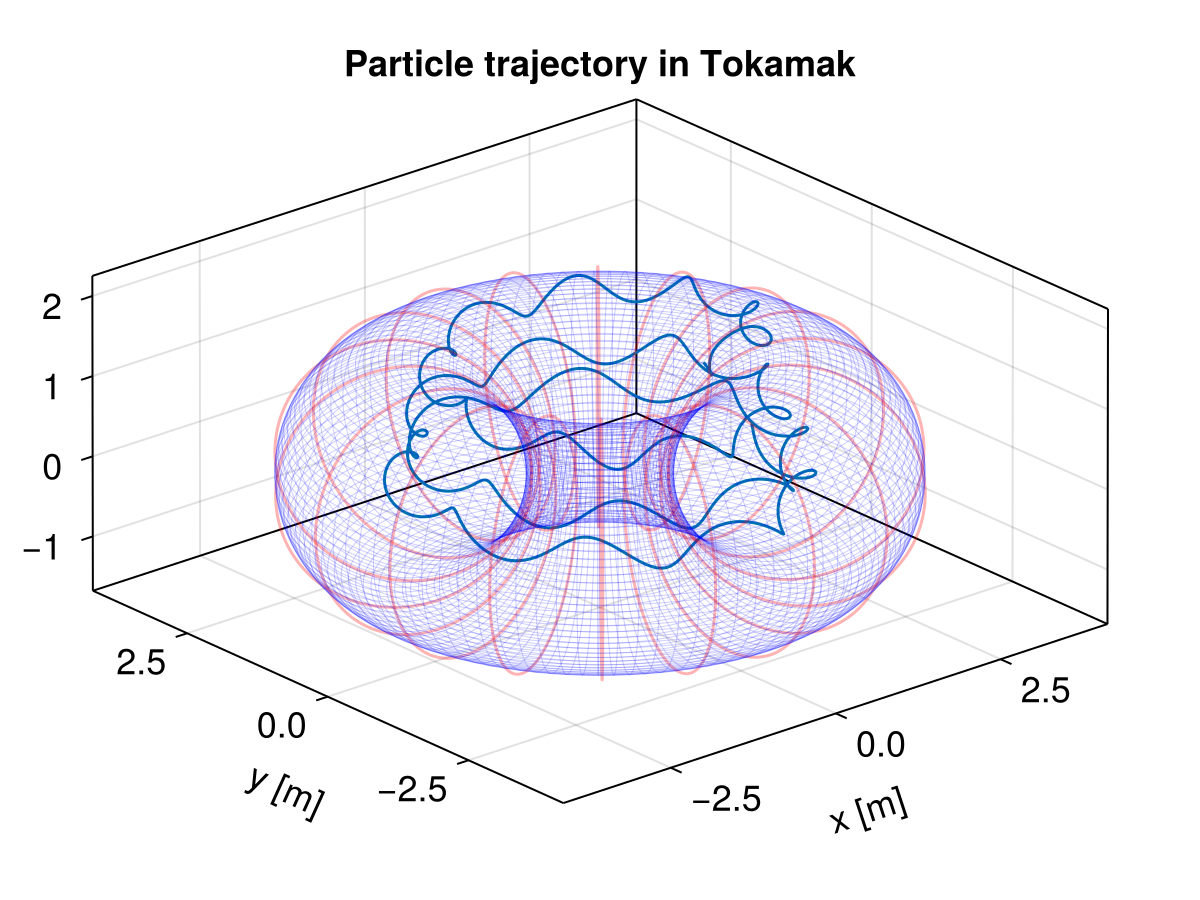
Coil Tokamak

This example shows how to trace protons in a stationary magnetic field that corresponds to a Tokamak represented by a circle of coils. A excellent introduction video to Tokamak can be found here in Mandarin.

julia

using TestParticle, OrdinaryDiffEqVerner, StaticArrays
import TestParticle as TP
using Statistics: mean
using Printf
using CairoMakie

### Obtain field

# Magnetic bottle parameters in SI units
const ICoil = 80.0 # current in the coil
const N = 15000 # number of windings
const IPlasma = 1.0e6 # current in the plasma
const a = 1.5 # radius of each coil
const b = 0.8 # radius of central region

getB(xu) = SVector{3}(TP.getB_tokamak_coil(xu[1], xu[2], xu[3], a, b, ICoil * N, IPlasma))

getE = TP.ZeroField()

### Initialize particles
m = TP.mᵢ
q = TP.qᵢ
c = TP.c

# initial velocity, [m/s]
v₀ = [-0.1, -0.15, 0.0] .* c
# initial position, [m]
r₀ = [2.3, 0.0, 0.0]
stateinit = [r₀..., v₀...]

param = prepare(getE, getB; species = Proton)
tspan = (0.0, 1.0e-6)

prob = ODEProblem(trace!, stateinit, tspan, param)

@printf "Speed = %6.4f %s\n" √(v₀[1]^2 + v₀[2]^2 + v₀[3]^2) / c * 100 "% speed of light"
@printf "Energy = %6.4f MeV\n" (1 / √(1 - (v₀[1] / c)^2 - (v₀[2] / c)^2 - (v₀[3] / c)^2) - 1) * m * c^2 / abs(q) / 1.0e6

# Default Tsit5() alone does not work in this case! You need to set a maximum
# timestep to maintain stability, or choose a different algorithm as well.
# The sample figure in the gallery is generated with AB3() and dt=2e-11.
sol = solve(prob, Vern9(); dt = 2.0e-11)

### Visualization

f = Figure(fontsize = 18)
ax = Axis3(
    f[1, 1],
    title = "Particle trajectory in Tokamak",
    xlabel = "x [m]",
    ylabel = "y [m]",
    zlabel = "z [m]",
    aspect = :data
)

lines!(ax, sol; idxs = (1, 2, 3), label = "proton")

# Plot coils
θ = range(0, 2π, length = 201)
y = a * cos.(θ)
z = a * sin.(θ)
for i in 0:17
    ϕ = i * π / 9
    lines!(ax, y * sin(ϕ) .+ (a + b) * sin(ϕ), y * cos(ϕ) .+ (a + b) * cos(ϕ), z, color = (:red, 0.3))
end

# Plot Tokamak
u = range(0, 2π, length = 100)
v = range(0, 2π, length = 100)

U = [y for _ in u, y in v]
V = [x for x in u, _ in v]

X = @. (a + b + (a - 0.05) * cos(U)) * cos(V)
Y = @. (a + b + (a - 0.05) * cos(U)) * sin(V)
Z = @. (a - 0.05) * sin(U)

wireframe!(ax, X, Y, Z, color = (:blue, 0.1), linewidth = 0.5, transparency = true)

Coil Tokamak ​

Coil Tokamak