Current Sheet

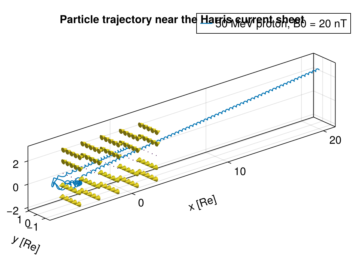
This example shows how to trace protons in a stationary magnetic field that corresponds to the 1D Harris current sheet defined by a reference strength and width. A Wiki reference can be found here.

using TestParticle, OrdinaryDiffEqVerner, StaticArrays
import TestParticle as TP
using TestParticle: Rₑ
using LinearAlgebra: norm
using CairoMakie

### Obtain field

# Harris current sheet parameters in SI units. Bn is the z-component.
const B₀, Bn, L = 20.0e-9, 2.0e-9, 0.4Rₑ

const getB = TP.HarrisCurrentSheet(B₀, L, Bn)

getE(xu) = SA[0.0, 0.0, 0.0]

### Initialize particles

# Initial condition
stateinit = let
    # initial particle energy, [eV]
    Ek = 8.0e3
    # initial velocity, [m/s]
    vmag = TP.c * √(1 - 1 / (1 + Ek * TP.qᵢ / (TP.mᵢ * TP.c^2))^2)
    θ = -60
    ϕ = 30
    v₀ = [vmag * cosd(θ), vmag * sind(θ) * sind(ϕ), vmag * sind(θ) * cosd(ϕ)]
    # initial position, [m]
    r₀ = [1Rₑ, 0Rₑ, 1Rₑ]

    [r₀..., v₀...]
end

param = prepare(getE, getB)
tspan = (0.0, -400.0)

prob = ODEProblem(trace!, stateinit, tspan, param)

sol = solve(prob, Vern9())

### Visualization

f = Figure(fontsize = 18)
ax = Axis3(
    f[1, 1],
    title = "Particle trajectory near the Harris current sheet",
    xlabel = "x [Re]",
    ylabel = "y [Re]",
    zlabel = "z [Re]",
    aspect = :data
)

n = 2000 # number of timepoints
ts = range(tspan..., length = n)
x = sol(ts, idxs = 1) ./ Rₑ |> Vector
y = sol(ts, idxs = 2) ./ Rₑ |> Vector
z = sol(ts, idxs = 3) ./ Rₑ |> Vector

l = lines!(ax, x, y, z, label = "50 MeV proton, B0 = 20 nT")
axislegend(ax, backgroundcolor = :transparent)

function plot_B!(ax)
    xrange = range(-5, 3, length = 5)
    yrange = range(-1, 1, length = 5)
    zrange = range(-2, 2, length = 5)

    ps = [Point3f(x, y, z) for x in xrange for y in yrange for z in zrange]
    B = map(p -> Vec3f(getB(p .* Rₑ) ./ B₀), ps)
    Bmag = norm.(B)

    return arrows!(ax, ps, B, fxaa = true, color = Bmag, lengthscale = 0.4, arrowsize = 0.05)
end

plot_B!(ax)