Performance Benchmark

This example compares the performance of the native Boris method against various ODE solvers from OrdinaryDiffEq.jl. We use Chairmarks.jl for benchmarking.

using Chairmarks
using TestParticle
using OrdinaryDiffEq
using GeometricIntegratorsDiffEq
using StaticArrays
using CairoMakie
using Statistics
using Random
import TestParticle as TP

Simulation Setup

We use a simple setup: an electron in a uniform magnetic field.

const Bmag = 0.01
uniform_B(x) = SA[0.0, 0.0, Bmag]
zero_E = ZeroField()

x0 = SA[0.0, 0.0, 0.0]
v0 = SA[0.0, 1.0e5, 0.0]
stateinit = SA[x0..., v0...]
# (q2m, m, E, B, F)
param = prepare(zero_E, uniform_B, species = Electron)
q2m = TP.get_q2m(param)

# Reference parameters
const tperiod = 2π / (abs(q2m) * Bmag)

tspan = (0.0, 400 * tperiod)
dt = tperiod / 12

prob_boris = TraceProblem(stateinit, tspan, param)
# ODE solvers from DifferentialEquations.jl are optimized for StaticArrays (SVector)
prob_ode = ODEProblem(trace, stateinit, tspan, param)
# GeometricIntegratorsDiffEq.jl requires mutable arrays
prob_gi = ODEProblem(trace, Vector(stateinit), tspan, param)

ODEProblem with uType Vector{Float64} and tType Float64. In-place: false
Non-trivial mass matrix: false
timespan: (0.0, 1.428954701151284e-6)
u0: 6-element Vector{Float64}:
      0.0
      0.0
      0.0
      0.0
 100000.0
      0.0

Benchmark

We benchmark the following solvers:

solvers = [
    ("Boris (n=1, N=2)", "standard Boris (n=1, N=2)", :Boris, () -> TP.solve(prob_boris; dt, n = 1, N = 2)),
    ("Boris (n=2, N=2)", "2-cycled (n=2, N=2)", :Boris, () -> TP.solve(prob_boris; dt, n = 2, N = 2)),
    ("Boris (n=4, N=2)", "4-cycled (n=4, N=2)", :Boris, () -> TP.solve(prob_boris; dt, n = 4, N = 2)),
    ("Boris (n=1, N=6)", "6-th order Boris (n=1, N=6)", :Boris, () -> TP.solve(prob_boris; dt, n = 1, N = 6)),
    ("Boris (n=2, N=6)", "Hyper Boris (n=2, N=6)", :Boris, () -> TP.solve(prob_boris; dt, n = 2, N = 6)),
    ("Boris (n=4, N=6)", "Hyper Boris (n=4, N=6)", :Boris, () -> TP.solve(prob_boris; dt, n = 4, N = 6)),
    ("Tsit5 (fixed)", "`OrdinaryDiffEq` Tsit5 with fixed step", :Fixed, () -> solve(prob_ode, Tsit5(); adaptive = false, dt, dense = false)),
    ("Tsit5 (adaptive)", "`OrdinaryDiffEq` Tsit5 with adaptive step", :Adaptive, () -> solve(prob_ode, Tsit5(); saveat = dt)),
    ("Vern7 (fixed)", "`OrdinaryDiffEq` Vern7 with fixed step", :Fixed, () -> solve(prob_ode, Vern7(); adaptive = false, dt, dense = false)),
    ("Vern7 (adaptive)", "`OrdinaryDiffEq` Vern7 with adaptive step", :Adaptive, () -> solve(prob_ode, Vern7(); saveat = dt)),
    ("Vern9 (fixed)", "`OrdinaryDiffEq` Vern9 with fixed step", :Fixed, () -> solve(prob_ode, Vern9(); adaptive = false, dt, dense = false)),
    ("Vern9 (adaptive)", "`OrdinaryDiffEq` Vern9 with adaptive step", :Adaptive, () -> solve(prob_ode, Vern9(); saveat = dt)),
    ("AutoVern7 (adaptive)", "`OrdinaryDiffEq` AutoVern7 with adaptive step", :Adaptive, () -> solve(prob_ode, AutoVern7(Rodas5()); saveat = dt)),
    ("AutoVern9 (adaptive)", "`OrdinaryDiffEq` AutoVern9 with adaptive step", :Adaptive, () -> solve(prob_ode, AutoVern9(Rodas5()); saveat = dt)),
    ("ImplicitMidpoint", "`OrdinaryDiffEq` ImplicitMidpoint with fixed step", :Fixed, () -> solve(prob_ode, ImplicitMidpoint(); adaptive = false, dt, dense = false)),
    ("GIEuler", "GeometricIntegrators Euler", :GI, () -> solve(prob_gi, GIEuler(); dt)),
    ("GIMidpoint", "GeometricIntegrators Midpoint", :GI, () -> solve(prob_gi, GIMidpoint(); dt)),
    ("GIRK4", "GeometricIntegrators RK4", :GI, () -> solve(prob_gi, GIRK4(); dt)),
]

Solver	Description
Boris (n=1, N=2)	standard Boris (n=1, N=2)
Boris (n=2, N=2)	2-cycled (n=2, N=2)
Boris (n=4, N=2)	4-cycled (n=4, N=2)
Boris (n=1, N=6)	6-th order Boris (n=1, N=6)
Boris (n=2, N=6)	Hyper Boris (n=2, N=6)
Boris (n=4, N=6)	Hyper Boris (n=4, N=6)
Tsit5 (fixed)	OrdinaryDiffEq Tsit5 with fixed step
Tsit5 (adaptive)	OrdinaryDiffEq Tsit5 with adaptive step
Vern7 (fixed)	OrdinaryDiffEq Vern7 with fixed step
Vern7 (adaptive)	OrdinaryDiffEq Vern7 with adaptive step
Vern9 (fixed)	OrdinaryDiffEq Vern9 with fixed step
Vern9 (adaptive)	OrdinaryDiffEq Vern9 with adaptive step
AutoVern7 (adaptive)	OrdinaryDiffEq AutoVern7 with adaptive step
AutoVern9 (adaptive)	OrdinaryDiffEq AutoVern9 with adaptive step
ImplicitMidpoint	OrdinaryDiffEq ImplicitMidpoint with fixed step
GIEuler	GeometricIntegrators Euler
GIMidpoint	GeometricIntegrators Midpoint
GIRK4	GeometricIntegrators RK4

To simulate realistic applications, we save the solution at fixed intervals for all solvers. For adaptive solvers, the default relative tolerance is 1e-3 and absolute tolerance is 1e-6.

"""
Helper functions to extract the median execution time and memory allocation.
"""
function get_median_time_memory(b)
    mb = median(b)
    return mb.time, mb.bytes
end

n_solvers = length(solvers)
results_time = Vector{Float64}(undef, n_solvers)
results_mem = Vector{Float64}(undef, n_solvers)
names = Vector{String}(undef, n_solvers)
groups = Vector{Symbol}(undef, n_solvers)

for (i, (name, desc, group, func)) in enumerate(solvers)
    println("Benchmarking $name...")
    b = @be $func() seconds = 1
    mt, mm = get_median_time_memory(b)
    results_time[i] = mt
    results_mem[i] = mm
    names[i] = name
    groups[i] = group
end

Benchmarking Boris (n=1, N=2)...
Benchmarking Boris (n=2, N=2)...
Benchmarking Boris (n=4, N=2)...
Benchmarking Boris (n=1, N=6)...
Benchmarking Boris (n=2, N=6)...
Benchmarking Boris (n=4, N=6)...
Benchmarking Tsit5 (fixed)...
Benchmarking Tsit5 (adaptive)...
Benchmarking Vern7 (fixed)...
Benchmarking Vern7 (adaptive)...
Benchmarking Vern9 (fixed)...
Benchmarking Vern9 (adaptive)...
Benchmarking AutoVern7 (adaptive)...
Benchmarking AutoVern9 (adaptive)...
Benchmarking ImplicitMidpoint...
Benchmarking GIEuler...
Benchmarking GIMidpoint...
Benchmarking GIRK4...

Normalize results

min_time = minimum(results_time)
min_mem = minimum(results_mem)

results_time_norm = results_time ./ min_time
results_mem_norm = results_mem ./ min_mem;

Detailed Performance Comparison

First, we present a detailed comparison of elapsed time and memory allocations for the solvers as a bar plot.

colors = Makie.wong_colors()

f = Figure(size = (1200, 800), fontsize = 24)

y_positions = 1:n_solvers

ax_time = Axis(
    f[1, 1],
    xlabel = "Elapsed Time (s)",
    ylabel = "Solvers",
    yticks = (y_positions, names),
    xscale = log10,
    xgridstyle = :dash,
    ygridstyle = :dash,
    xminorticksvisible = true,
    xminorticks = IntervalsBetween(9)
)

ax_mem = Axis(
    f[1, 1],
    xaxisposition = :top,
    xlabel = "Memory Allocations (kB)",
    xscale = log10,
    xgridvisible = false,
    ygridvisible = false,
    yticksvisible = false,
    yticklabelsvisible = false,
    xminorticksvisible = true,
    xminorticks = IntervalsBetween(9)
)

linkyaxes!(ax_time, ax_mem)

bar_width = 0.35
color_time = colors[1]
color_mem = colors[2]

barplot!(
    ax_time, y_positions .- bar_width / 2, results_time;
    direction = :x, width = bar_width, color = color_time
)

# Avoid 0 for log plot
results_mem_kb = results_mem ./ 1024
safe_results_mem = max.(results_mem_kb, 1.0e-3)
barplot!(
    ax_mem, y_positions .+ bar_width / 2, safe_results_mem;
    direction = :x, width = bar_width, color = color_mem
)

elements = [PolyElement(polycolor = color_time), PolyElement(polycolor = color_mem)]
labels = ["Elapsed Time", "Memory Allocations"]
Legend(
    f[1, 1], elements, labels, "Metrics";
    framevisible = false, halign = :right, valign = :bottom,
    tellwidth = false, tellheight = false
)

Solver Efficiency

Next, we evaluate the solver efficiency by plotting relative time versus relative memory.

f2 = Figure(size = (1200, 800), fontsize = 24)

ax = Axis(
    f2[1, 1],
    title = "Solver Efficiency (Time vs. Memory)",
    xlabel = "Relative Time (1.0 = Fastest)",
    ylabel = "Relative Memory (1.0 = Lowest)",
    xgridstyle = :dash,
    ygridstyle = :dash,
    xscale = log10,
    yscale = log10,
    xminorticksvisible = true,
    yminorticksvisible = true,
    xminorticks = IntervalsBetween(9),
    yminorticks = IntervalsBetween(9)
)

Makie.Axis with 0 plots:

Defined groups and colors

unique_groups = unique(groups)
group_colors = Dict(g => colors[i] for (i, g) in enumerate(unique_groups))

Dict{Symbol, ColorTypes.RGBA{Float32}} with 4 entries:
  :Boris    => RGBA(0.0, 0.447059, 0.698039, 1.0)
  :Adaptive => RGBA(0.0, 0.619608, 0.45098, 1.0)
  :Fixed    => RGBA(0.901961, 0.623529, 0.0, 1.0)
  :GI       => RGBA(0.8, 0.47451, 0.654902, 1.0)

Marker palette for the individual solvers in each group

marker_palette = [:circle, :rect, :utriangle, :dtriangle, :diamond, :pentagon, :hexagon, :star5, :xcross, :cross]

legend_elements = Vector{Vector{MarkerElement}}()
legend_labels = Vector{Vector{String}}()
legend_titles = String[]

for g in unique_groups
    idxs = findall(==(g), groups)
    group_elements = MarkerElement[]
    group_labels = String[]
    for (i, idx) in enumerate(idxs)
        marker_shape = marker_palette[mod1(i, length(marker_palette))]
        push!(
            group_elements,
            MarkerElement(
                color = (group_colors[g], 0.7), marker = marker_shape,
                markersize = 15, strokecolor = :black, strokewidth = 1
            )
        )
        push!(group_labels, names[idx])

        scatter!(
            ax, [results_time_norm[idx]], [results_mem_norm[idx]],
            color = (group_colors[g], 0.7),
            marker = marker_shape,
            markersize = 25,
            strokewidth = 1,
            strokecolor = :black
        )
    end
    push!(legend_elements, group_elements)
    push!(legend_labels, group_labels)
    push!(legend_titles, string(g))
end

Add Legend outside the plot

Legend(f2[1, 2], legend_elements, legend_labels, legend_titles, framevisible = false)

# Highlight the "Utopia Point" (Theoretical Best)
scatter!(
    ax, [1.0], [1.0],
    marker = :star5,
    markersize = 20,
    color = (:red, 0.7),
    label = "Ideal Limit"
)
text!(
    ax, 1.0, 1.0, text = "Utopia Point", align = (:right, :top),
    offset = (55, -5), color = :red, fontsize = 15
)

# Add "Iso-Efficiency" curves (Optional visual aid)
# Curves where Time * Memory = Constant (Cost invariant)
x_range = range(
    minimum(results_time_norm) * 0.8, stop = maximum(results_time_norm) * 1.1, length = 100
)
lines!(ax, x_range, 5.0 ./ x_range, color = (:gray, 1.0), linestyle = :dot)
text!(
    ax, maximum(x_range), 5.0 / maximum(x_range),
    text = "Iso-cost", fontsize = 20, color = :black
)

xlims!(ax, minimum(results_time_norm) * 0.5, maximum(results_time_norm) * 1.5)
ylims!(ax, minimum(results_mem_norm) * 0.5, maximum(results_mem_norm) * 1.5)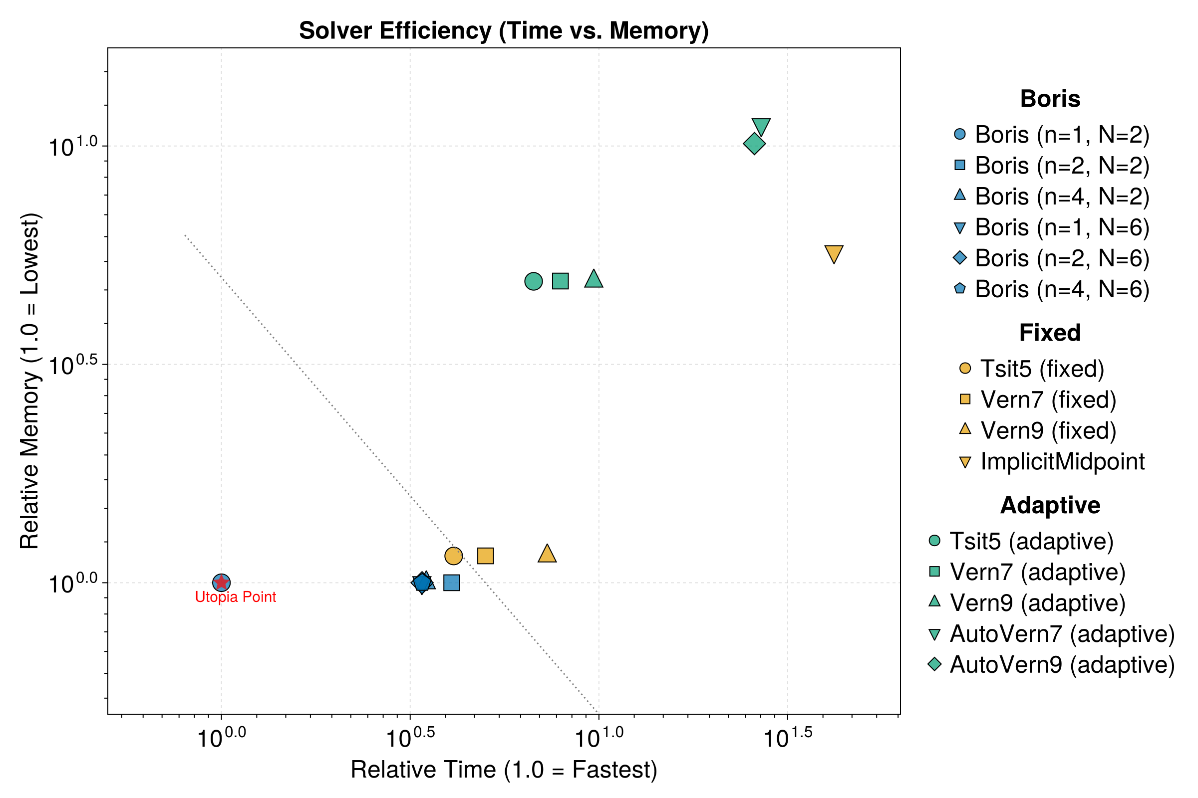

In practice, it is pretty hard to find an optimal algorithm. The native Boris method is good if you want a fixed time step. When calling OrdinaryDiffEq.jl, we recommend using Vern9() as a starting point instead of Tsit5(), especially combined with adaptive timestepping. Further fine-grained control includes setting dtmax, reltol, and abstol in the solve method.