ExB Drift

This example demonstrates a single proton motion under uniform E and B fields. The electric field is parallel to the magnetic field in the z-direction, so the motion consists of a cyclotron gyration and an acceleration along z. On top of that, particles also exhibit an ExB drift in the direction perpendicular to both E and B field. More theoretical details can be found in ExB Drift.

using TestParticle, OrdinaryDiffEq, StaticArrays
using CairoMakie

Plotting Function

We define a function to visualize the results for different drift cases.

function plot_exb_case(sol, sol_gc, title; layout = :three_columns)
    fig_size = layout == :three_columns ? (1600, 600) : (1200, 800)
    fig = Figure(size = fig_size, fontsize = 20)

    # 1. Left Column: Time Series
    gl_left = fig[1, 1] = GridLayout()
    ax_pos = Axis(gl_left[1, 1], ylabel = "Position [m]", title = title)
    lines!(ax_pos, sol, idxs = (0, 1), label = "x")
    lines!(ax_pos, sol, idxs = (0, 2), label = "y")
    lines!(ax_pos, sol, idxs = (0, 3), label = "z")
    axislegend(ax_pos, position = :lt, framevisible = true, backgroundcolor = (:white, 0.5))
    hidexdecorations!(ax_pos, grid = false)

    ax_vel = Axis(gl_left[2, 1], xlabel = "Time [s]", ylabel = "Velocity [m/s]")
    lines!(ax_vel, sol, idxs = (0, 4), label = "vx")
    lines!(ax_vel, sol, idxs = (0, 5), label = "vy")
    lines!(ax_vel, sol, idxs = (0, 6), label = "vz")
    axislegend(ax_vel, position = :lt, framevisible = true, backgroundcolor = (:white, 0.5))

    linkxaxes!(ax_pos, ax_vel)

    # 2. Trajectories
    if layout == :three_columns
        ax_3d = Axis3(
            fig[1, 2];
            title = "3D Trajectory", xlabel = "x", ylabel = "y", zlabel = "z", aspect = :data
        )
        gl_right = fig[1, 3] = GridLayout()
        ax_2d = Axis(
            gl_right[1, 1];
            title = "Y-X Plane Trajectory", xlabel = "y", ylabel = "x", aspect = DataAspect()
        )
        cbar_pos = gl_right[1, 2]
    else
        gl_right = fig[1, 2] = GridLayout()
        ax_3d = Axis3(
            gl_right[1, 1];
            title = "3D Trajectory", xlabel = "x", ylabel = "y", zlabel = "z", aspect = :data
        )
        ax_2d = Axis(
            gl_right[2, 1];
            title = "Y-X Plane Trajectory", xlabel = "y", ylabel = "x", aspect = DataAspect()
        )
        cbar_pos = gl_right[2, 2]
    end

    lines!(ax_3d, sol, idxs = (1, 2, 3), color = :black, alpha = 0.5, label = "Particle")
    lines!(ax_3d, sol_gc, idxs = (1, 2, 3), color = :red, linewidth = 3, label = "GC")
    axislegend(ax_3d, framevisible = true, backgroundcolor = (:white, 0.5))

    lines!(ax_2d, sol, idxs = (2, 1), color = :black, alpha = 0.5, label = "Particle")
    lines!(ax_2d, sol_gc, idxs = (2, 1), color = :red, linewidth = 2, label = "GC")

    q2m = sol.prob.p[1]
    energy_func(x, y, z, vx, vy, vz) = 0.5 * (vx^2 + vy^2 + vz^2) / q2m
    t_sampled = range(sol.t[1], sol.t[end], length = 200)
    sol_sampled = sol(t_sampled)
    y_s = sol_sampled[2, :]
    x_s = sol_sampled[1, :]
    energy_s = [energy_func(u...) for u in sol_sampled.u]

    sc = scatter!(ax_2d, y_s, x_s, color = energy_s, colormap = :Spectral, markersize = 6)
    Colorbar(cbar_pos, sc, label = "Energy [eV]")
    axislegend(ax_2d, position = :rt, framevisible = true, backgroundcolor = (:white, 0.5))

    return fig
end

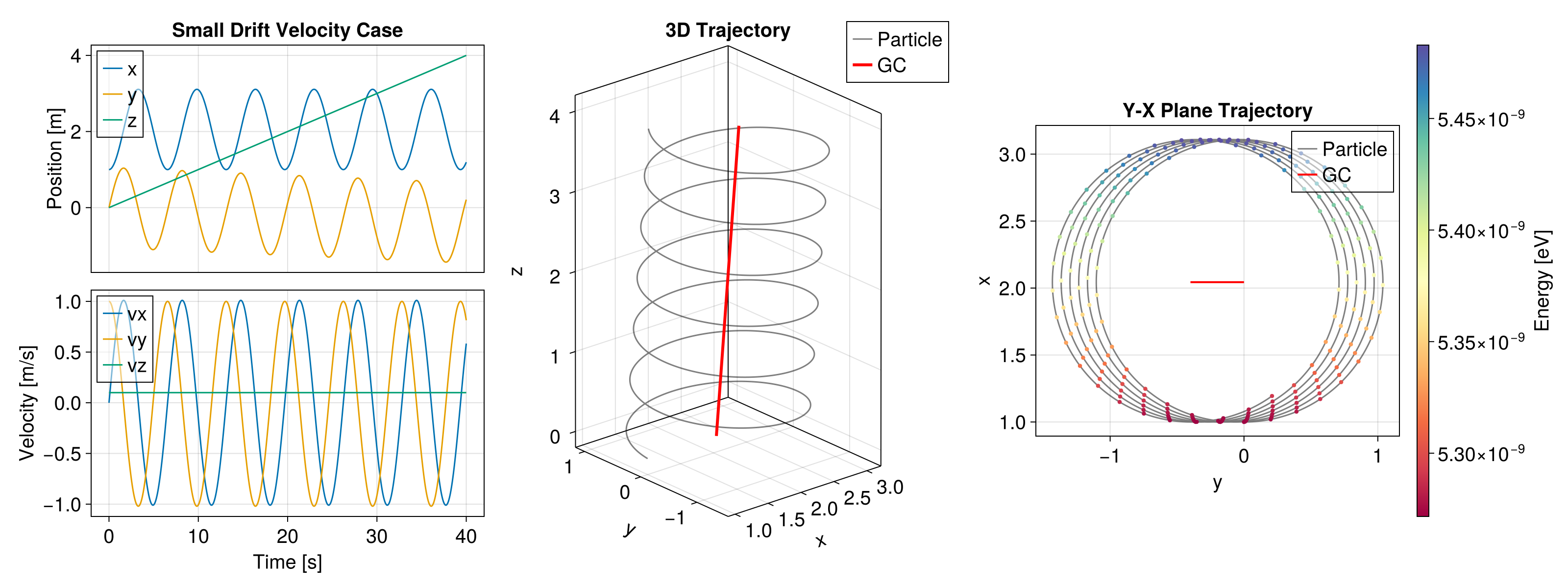
plot_exb_case (generic function with 1 method)

Small Drift Velocity

In this case, the drift velocity $V_d=E/B$ is much smaller than the initial perpendicular velocity $V_{\perp }$. The trajectory exhibits clear loops.

# Analytic EM fields
uniform_B(x) = SA[0, 0, 1.0e-8]
uniform_E_small(x) = SA[1.0e-10, 0, 0]

# Initial condition: [x, y, z, vx, vy, vz]
stateinit_small = [1.0, 0.0, 0.0, 0.0, 1.0, 0.1]
tspan = (0, 40)

param_small = prepare(uniform_E_small, uniform_B, species = Proton)
prob_small = ODEProblem(trace!, stateinit_small, tspan, param_small)
sol_small = solve(prob_small, Vern9())

# Tracing guiding center
gc_small = param_small |> get_gc_func
gc_x0_small = gc_small(stateinit_small) |> Vector
prob_gc_small = ODEProblem(trace_gc_exb!, gc_x0_small, tspan, (param_small..., sol_small))
sol_gc_small = solve(prob_gc_small, Vern9(); save_idxs = [1, 2, 3])

fig_small = plot_exb_case(
    sol_small, sol_gc_small, "Small Drift Velocity Case";
    layout = :three_columns
)

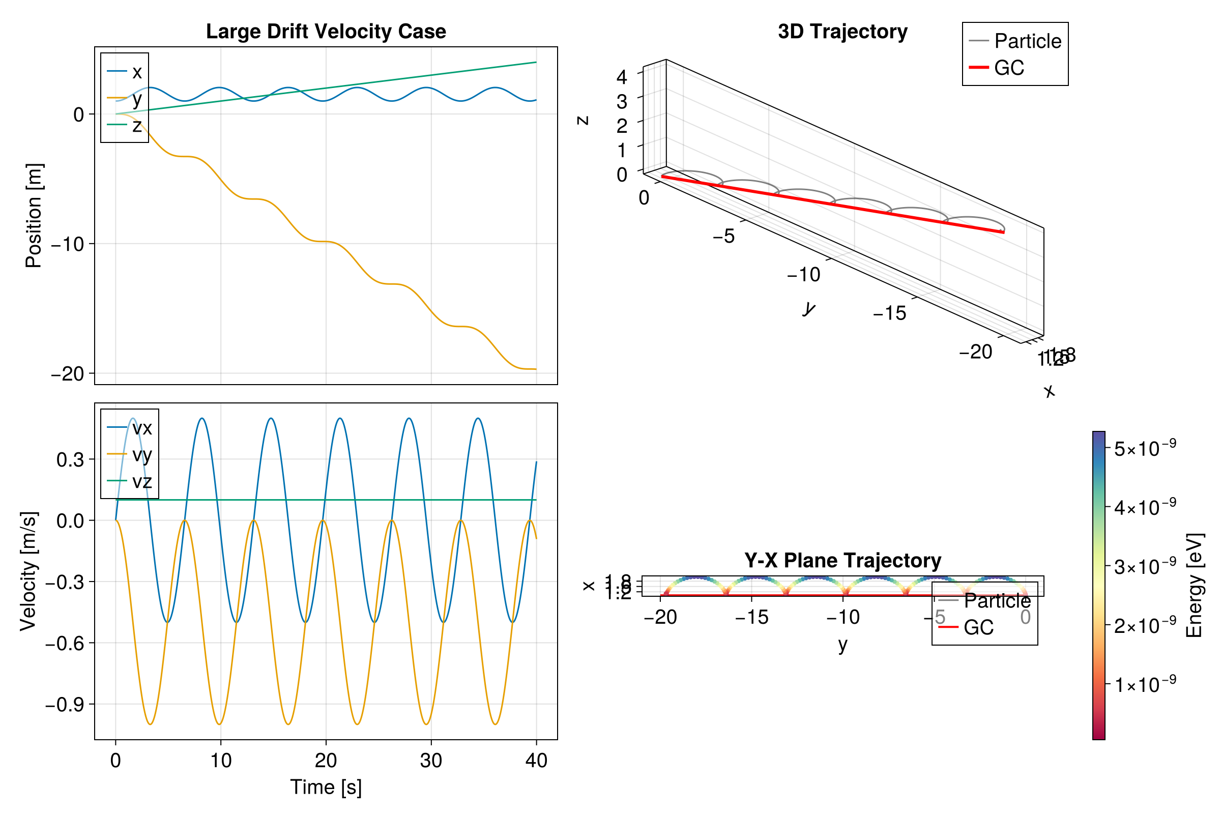
Large Drift Velocity

In this case, the drift velocity $V_d$ is comparable to the initial velocity. We use $V_y=0$ at $t=0$ to demonstrate a cycloid with cusps.

uniform_E_large(x) = SA[5.0e-9, 0, 0]
stateinit_large = [1.0, 0.0, 0.0, 0.0, 0.0, 0.1]

param_large = prepare(uniform_E_large, uniform_B, species = Proton)
prob_large = ODEProblem(trace!, stateinit_large, tspan, param_large)
sol_large = solve(prob_large, Vern9())

gc_large = param_large |> get_gc_func
gc_x0_large = gc_large(stateinit_large) |> Vector
prob_gc_large = ODEProblem(trace_gc_exb!, gc_x0_large, tspan, (param_large..., sol_large))
sol_gc_large = solve(prob_gc_large, Vern9(); save_idxs = [1, 2, 3])

fig_large = plot_exb_case(
    sol_large, sol_gc_large, "Large Drift Velocity Case";
    layout = :two_columns
)