Solver Accuracy Analysis
This example demonstrates how to analyze the accuracy of different Boris particle solvers. We compare the standard Boris method, the Multicycle Boris method, and the Hyper Boris method proposed in Zenitani & Kato (2025).
Two test cases are presented: 2. Phase Error in Circular Motion: A particle in a uniform magnetic field and zero electric field. We measure the phase error in velocity over multiple periods.
- Velocity Error in Static E and B Fields: A particle in uniform magnetic and electric fields. We measure the maximum error in velocity compared to the analytical solution.
!! IMPORTANT Note that while the original Boris solver's gyrophase correction [4] only corrects the magnetic field, our implementation of the Hyper Boris solver (
using TestParticle
using OrdinaryDiffEq, OrdinaryDiffEqLowOrderRK
using StaticArrays
using LinearAlgebra
using CairoMakie
Solvers to Test
We define a set of Boris solvers and ODE solvers to compare.
boris_solvers = [
    ("Standard Boris", Boris()),
    ("Multicycle Boris (n=2)", MultistepBoris2(; n = 2)),
    ("Multicycle Boris (n=4)", MultistepBoris2(; n = 4)),
    ("Hyper Boris (n=1, N=6)", MultistepBoris6(; n = 1)),
    ("Hyper Boris (n=2, N=6)", MultistepBoris6(; n = 2)),
    ("Hyper Boris (n=4, N=4)", MultistepBoris4(; n = 4)),
    ("Hyper Boris (n=4, N=6)", MultistepBoris6(; n = 4)),
]

ode_solvers = [
    ("RK4", RK4()),
    ("Tsit5", Tsit5()),
    ("Vern6", Vern6()),
]

# Generic reference line plotting function
function plot_ref_line!(ax, dts, errors, order; offset = 1.5, color = :black, idxt = 1)
    suffix = order == 2 ? "nd" : order == 3 ? "rd" : "th"
    # Align with the error at the smallest dt to ensure it's visible above the data
    dt_min, idx_min = findmin(dts)
    ref_y = offset .* errors[idx_min] .* (dts ./ dt_min) .^ order
    l = lines!(ax, dts, ref_y, linestyle = :dash, color = color)

    # Add text label on top of the line
    # Use the provided index for placement. Default is 1 (smallest dt).
    # Adjust rotation to match the visual slope in log-log space.
    # Based on the axis aspect ratio, a factor is needed.
    rotation = atan(order / 7.5)
    text!(
        ax, dts[idxt], ref_y[idxt], text = "$(order)$suffix order",
        color = color, align = (:left, :bottom), offset = (5, 5),
        rotation = rotation
    )
    return l
end
plot_ref_line! (generic function with 1 method)Section 1: Phase Error Analysis
In a uniform magnetic field with no electric field, a particle undergoes circular motion (cyclotron motion). We analyze the accumulated phase error in velocity.
# Test Problem Definition
B_func(x, t) = SA[0.0, 0.0, 1.0]
E_func = ZeroField()

# Parameters (Dimensionless units: q=1, m=1, B=1)
q = 1.0
m = 1.0
Ω = q * 1.0 / m       # Cyclotron frequency
T_period = 2π / Ω     # Cyclotron period

# Initial condition
x0 = [0.0, 0.0, 0.0]
v0 = [1.0, 0.0, 0.0]
u0 = [x0..., v0...]

# Simulation time
n_periods = 10
t_end = n_periods * T_period
tspan = (0.0, t_end)

# Trace problem
param = prepare(E_func, B_func; q, m)
prob1 = TraceProblem(u0, tspan, param)

# Time steps to test
steps_per_period1 = [10, 20, 40, 80, 160, 320]
dts1 = T_period ./ steps_per_period1

# Storage for results
results1 = Dict(name => Float64[] for (name, _) in [boris_solvers; ode_solvers])

# ODE problem
prob1_ode = ODEProblem(trace!, u0, tspan, param)

for dt in dts1
    for (name, alg) in boris_solvers
        sol = TestParticle.solve(prob1, alg; dt).u[1]
        vx, vy = sol.u[end][4], sol.u[end][5]
        t_final = sol.t[end]

        phi_num = atan(vy, vx)
        phi_ana = -Ω * t_final

        push!(results1[name], abs(rem2pi(phi_num - phi_ana, RoundNearest)))
    end
    for (name, alg) in ode_solvers
        sol = OrdinaryDiffEq.solve(prob1_ode, alg; adaptive = false, dt, saveat = dt)
        vx, vy = sol.u[end][4], sol.u[end][5]
        t_final = sol.t[end]

        phi_num = atan(vy, vx)
        phi_ana = -Ω * t_final

        push!(results1[name], abs(rem2pi(phi_num - phi_ana, RoundNearest)))
    end
end
Section 2: Velocity Error in Static E and B Fields
We now test a more complex case from Section 6 of Zenitani & Kato (2025), where both magnetic and electric fields are non-zero.
# Test Problem Definition
B_func2(x, t) = SA[0.0, 0.0, 1.0]
E_func2(x, t) = SA[0.0, 0.5, 0.1]

# Parameters
q = 1.0
m = 1.0
ωc = q * 1.0 / m # Gyro frequency

# Initial condition: particle starting at origin with zero velocity
x0 = [0.0, 0.0, 0.0]
v0 = [0.0, 0.0, 0.0]
u0 = [x0..., v0...]

# Simulation time: 6 gyroperiods
t_end2 = 6 * (2π / ωc)
tspan2 = (0.0, t_end2)

# Exact solution function for constant E and B
function exact_velocity(t, E, B, q, m)
    Bmag = norm(B)
    b_hat = B / Bmag
    ωc = q * Bmag / m
    vD = (E × B) / Bmag^2
    E_parallel = (E ⋅ b_hat) * b_hat

    # For v(0) = 0
    v_perp = -vD * cos(ωc * t) - (vD × b_hat) * sin(ωc * t) + vD
    v_para = (q * E_parallel / m) * t
    return v_perp + v_para
end

# Trace problem
param2 = prepare(E_func2, B_func2; q, m)
prob2 = TraceProblem(u0, tspan2, param2)

# Time steps to test: from π/120 to π (log-spaced)
dts2 = logrange(π / 120, π, 10)

# Storage for results
results2 = Dict(name => Float64[] for (name, _) in [boris_solvers; ode_solvers])

# ODE problem
prob2_ode = ODEProblem(trace!, u0, tspan2, param2)

for dt in dts2
    for (name, alg) in boris_solvers
        sol = TestParticle.solve(prob2, alg; dt).u[1]

        max_err = 0.0
        for i in eachindex(sol.u)
            v_num = sol.u[i][4:6]
            v_ana = exact_velocity(sol.t[i], E_func2(nothing, 0), B_func2(nothing, 0), q, m)
            max_err = max(max_err, norm(v_num - v_ana))
        end
        push!(results2[name], max_err)
    end
    for (name, alg) in ode_solvers
        sol = OrdinaryDiffEq.solve(prob2_ode, alg; adaptive = false, dt, saveat = dt)

        max_err = 0.0
        for i in eachindex(sol.u)
            v_num = sol.u[i][4:6]
            v_ana = exact_velocity(sol.t[i], E_func2(nothing, 0), B_func2(nothing, 0), q, m)
            max_err = max(max_err, norm(v_num - v_ana))
        end
        push!(results2[name], max_err)
    end
end
Visualization
f = Figure(size = (1200, 500), fontsize = 20);

# Phase Error Plot
ax1 = Axis(
    f[1, 1],
    xscale = log10, yscale = log10,
    xlabel = L"Time step ($dt / T_\mathrm{gyro}$)",
    ylabel = "Phase Error (rad)",
    title = "Phase Error Convergence",
    xminorticksvisible = true, yminorticksvisible = true,
    xminorticks = IntervalsBetween(9), yminorticks = IntervalsBetween(9),
    xgridvisible = true, ygridvisible = true
)

for (name, _) in boris_solvers
    scatterlines!(
        ax1, dts1 ./ T_period, results1[name];
        label = name, linewidth = 2, marker = :circle
    )
end
for (name, _) in ode_solvers
    scatterlines!(
        ax1, dts1 ./ T_period, results1[name];
        label = name, linewidth = 2, marker = :cross
    )
end

plot_ref_line!(ax1, dts1 ./ T_period, results1["Standard Boris"], 2, color = :black, idxt = 6)
plot_ref_line!(ax1, dts1 ./ T_period, results1["Hyper Boris (n=4, N=4)"], 4, color = :red, idxt = 6)
plot_ref_line!(ax1, dts1 ./ T_period, results1["Tsit5"], 5, color = :orange, idxt = 6)
plot_ref_line!(ax1, dts1 ./ T_period, results1["Hyper Boris (n=4, N=6)"], 6, color = :gray, idxt = 6)

# Velocity Error Plot
ax2 = Axis(
    f[1, 2],
    xscale = log10, yscale = log10,
    xlabel = L"Time step ($dt / T_\mathrm{gyro}$)",
    ylabel = "Max Velocity Error",
    title = "Velocity Error Convergence",
    xminorticksvisible = true, yminorticksvisible = true,
    xminorticks = IntervalsBetween(9), yminorticks = IntervalsBetween(9),
    xgridvisible = true, ygridvisible = true
)

T_period2 = 2π / ωc

for (name, _) in boris_solvers
    scatterlines!(
        ax2, dts2 ./ T_period2, results2[name];
        label = name, linewidth = 2, marker = :circle
    )
end
for (name, _) in ode_solvers
    scatterlines!(
        ax2, dts2 ./ T_period2, results2[name];
        label = name, linewidth = 2, marker = :cross
    )
end

plot_ref_line!(ax2, dts2 ./ T_period2, results2["Standard Boris"], 2, color = :black, idxt = 1)
plot_ref_line!(ax2, dts2 ./ T_period2, results2["Hyper Boris (n=4, N=4)"], 4, color = :red, idxt = 1)
plot_ref_line!(ax2, dts2 ./ T_period2, results2["Tsit5"], 5, color = :orange, idxt = 1)
plot_ref_line!(ax2, dts2 ./ T_period2, results2["Hyper Boris (n=4, N=6)"], 6, color = :gray, idxt = 1)

f[1, 3] = Legend(f, ax2, framevisible = false)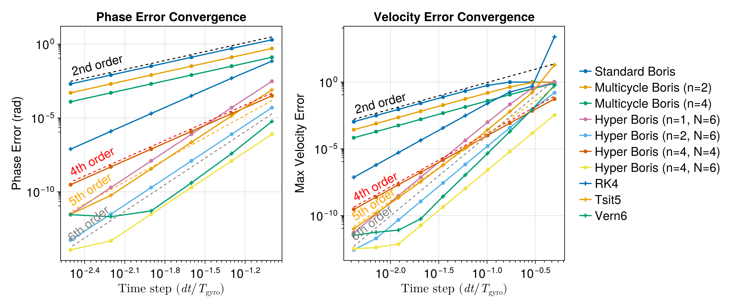
Order of Accuracy Estimation
function estimate_order(dts, errors)
    # Linear regression on log-log data
    X = [ones(length(dts)) log10.(dts)]
    Y = log10.(errors)
    return (X \ Y)[2]
end

println("Estimated Order of Accuracy (Velocity Error):")
for (name, _) in [boris_solvers; ode_solvers]
    slope = estimate_order(dts2, results2[name])
    println("$name: $(round(slope, digits = 2))")
end
Estimated Order of Accuracy (Velocity Error):
Standard Boris: 1.55
Multicycle Boris (n=2): 1.83
Multicycle Boris (n=4): 1.97
Hyper Boris (n=1, N=6): 5.66
Hyper Boris (n=2, N=6): 5.82
Hyper Boris (n=4, N=4): 3.99
Hyper Boris (n=4, N=6): 5.21
RK4: 4.4
Tsit5: 5.75
Vern6: 5.74Section 3: Long-term Drift Tracking
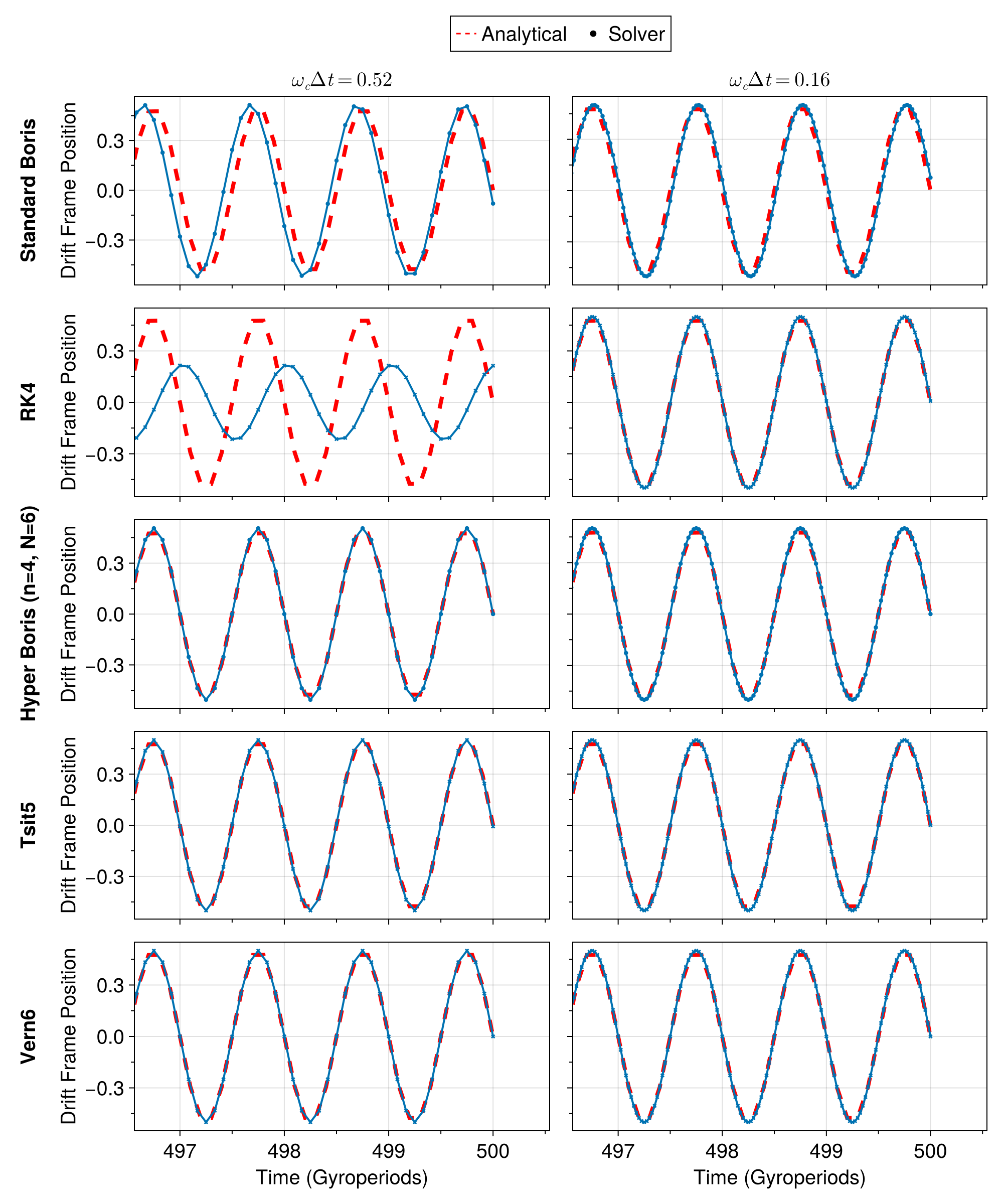
We check the long-term behaviors over many gyroperiods for a subset of solvers using two specific time steps:
drift_solvers_all = [
    ("Standard Boris", :boris, Boris()),
    ("RK4", :ode, RK4()),
    ("Hyper Boris (n=4, N=6)", :boris, MultistepBoris6(; n = 4)),
    ("Tsit5", :ode, Tsit5()),
    ("Vern6", :ode, Vern6()),
]

# Simulation time: 500 gyroperiods
t_end3 = 500 * (2π / ωc)
tspan3 = (0.0, t_end3)

# Exact analytical position in drift frame for E=(0, 0.5, 0.1), B=(0, 0, 1) and v(0)=0
# E x B / B^2 = (0.5, 0, 0), so drift is purely in +x direction.
# Exact position x(t) = v_D * t - (v_D / ωc) * sin(ωc * t)
# Drift frame x: x_drift(t) = x(t) - v_D * t = -(v_D / ωc) * sin(ωc * t)
vD_magnitude = 0.5
exact_x_drift(t) = -(vD_magnitude / ωc) * sin(ωc * t)

prob3 = TraceProblem(u0, tspan3, param2)
prob3_ode = ODEProblem(trace!, u0, tspan3, param2)

dts3 = [π / 6, π / 20]
t_exact_plot = range(0.0, t_end3, length = 5000)
x_drift_exact = exact_x_drift.(t_exact_plot)

f3 = Figure(size = (1000, 1200), fontsize = 20)

for (row, (name, type, config)) in enumerate(drift_solvers_all)
    for (col, dt) in enumerate(dts3)
        ax = Axis(
            f3[row, col],
            xlabel = row == length(drift_solvers_all) ? "Time (Gyroperiods)" : "",
            ylabel = col == 1 ? "Drift Frame Position" : "",
            title = row == 1 ? L"\omega_c \Delta t = %$(round(dt, digits = 2))" : "",
            xminorticksvisible = true, yminorticksvisible = true,
            xgridvisible = true, ygridvisible = true,
            xticklabelsvisible = row == length(drift_solvers_all),
            yticklabelsvisible = col == 1
        )

        # Add row title for the solver
        if col == 1
            Label(f3[row, 0], name, rotation = π / 2, font = :bold, tellheight = false)
        end

        # Plot analytical solution
        lines!(
            ax, t_exact_plot ./ T_period2, x_drift_exact;
            label = "Analytical", color = :red, linestyle = :dash, linewidth = 4
        )

        # Plot solver result
        if type == :boris
            sol = TestParticle.solve(prob3, config; dt).u[1]
            t_eval = range(0.0, t_end3, step = dt)
            x_drifts = [sol(t)[1] - vD_magnitude * t for t in t_eval]
            scatterlines!(
                ax, t_eval ./ T_period2, x_drifts;
                label = name, linewidth = 2, marker = :circle, markersize = 6
            )
        else
            sol = OrdinaryDiffEq.solve(prob3_ode, config; adaptive = false, dt, saveat = dt)
            x_drifts = [u[1] - vD_magnitude * t for (t, u) in zip(sol.t, sol.u)]
            scatterlines!(
                ax, sol.t ./ T_period2, x_drifts;
                label = name, linewidth = 2, marker = :xcross, markersize = 6
            )
        end

        xlims!(ax, [3120, 3145] ./ T_period2)
    end
end

# Add a single legend at the top
Legend(
    f3[0, 1:2], [
        LineElement(color = :red, linestyle = :dash),
        MarkerElement(marker = :circle, color = :black),
    ],
    ["Analytical", "Solver"],
    orientation = :horizontal, tellwidth = false, tellheight = true
)