Electron Fermi Acceleration Inside Foreshock Transient Cores

This example demonstrates electron acceleration via Fermi acceleration using a simple 1D model. It follows the setup described in Fermi acceleration of electrons inside foreshock transient cores. The simulation domain is $2 R_{E}$ in x, where the initial magnetosheath locates at $x \in [0, 0.5] R_{E}$ with a magnetic field $B_{z} = 20 nT$ and the bow shock at $x = 0.5 R_{E}$ . The foreshock transient boundary is at $x = 1.5 R_{E}$ initially and moves toward the bow shock at a speed $U = 100 km / s$ . The region beyond $x = 1.5 R_{E}$ is the foreshock transient sheath in which the magnetic field is $B_{z} = 10 nT$ . A convection electric field $E_{y} = - 1 mV / m$ , consistent with the velocity U, is introduced in the foreshock transient sheath. Between the two boundaries, $0.5 R_{E} < x < 1.5 R_{E}$ , is the foreshock transient's core region.

In the first case, the magnetic field in the core region is set to zero. In the second case, a magnetic fluctuation is imposed:

\begin{array}{r} δ B_{x, y, z} = \sum_{N = N_{0}}^{N_{1}} δ B_{N} \cos (\frac{2 π N x}{L_{0}} + ϕ_{x, y, z}^{N}) \\ δ B_{N} = \tilde{B} (N / N_{0})^{- 1.2}, N = N_{0}, N_{0} + 1, . . ., N_{1} \end{array}

Here $L_{0} = 1 R_{E}$ is the initial length of the core in the x direction. We choose $N_{0} = 100, N_{1} = 1000, \tilde{B} = 0.2 nT$ , and $ϕ_{x, y, z}^{N}$ as the random phases of various modes between 0 and 2π (independently different in the x, y, and z directions). As the low-frequency wave speed ( $\sim O (10) km / s$ ) is much smaller than the electron speed ( $\sim O (10^{3}) km / s$ ), we do not include wave propagation in this 1D model.

One important note about Fermi acceleration for space plasmas is that space plasmas are collisionless. Electric field is the only way to accelerate charged particles, instead of elastic collisions.

julia

using TestParticle, OrdinaryDiffEqVerner, StaticArrays
import TestParticle as TP
using TestParticle: mₑ, Rₑ, qₑ
using TestParticle: get_EField, get_BField
using Random
using FHist
using CairoMakie, Printf

# For reproducible results
Random.seed!(1234)

# Analytic EM fields

function Bcase1(xu, t)
    Bz = if xu[1] < 0.5Rₑ
        20.0e-9
    elseif xu[1] > 1.5Rₑ + U * t
        10.0e-9
    else
        0.0
    end

    return SA[0.0, 0.0, Bz]
end

function E(xu, t)
    Ey = if xu[1] > 1.5Rₑ + U * t
        -1.0e-3
    else
        0.0
    end

    return SA[0.0, Ey, 0.0]
end

Bcase2(xu, t) =
if xu[1] < 0.5Rₑ
    SA[0.0, 0.0, 20.0e-9]
elseif xu[1] > 1.5Rₑ + U * t
    SA[0.0, 0.0, 10.0e-9]
else
    δBfunc(xu)
end

function get_B_perturb(x)
    L₀, N₀, N₁, B̃ = 1Rₑ, 100, 1000, 0.2e-9
    B = fill(0.0, 3, length(x)) # [T]
    # Eqs (4-5) from the paper
    for N in N₀:N₁
        δBn = B̃ * (N / N₀)^-1.2
        ϕx, ϕy, ϕz = rand(SVector{3, Float64}) .* 2
        for i in axes(B, 2)
            δBx = δBn * cospi(2 * N * x[i] / L₀ + ϕx)
            δBy = δBn * cospi(2 * N * x[i] / L₀ + ϕy)
            δBz = δBn * cospi(2 * N * x[i] / L₀ + ϕz)
            B[1, i] += δBx
            B[2, i] += δBy
            B[3, i] += δBz
        end
    end

    return B
end

isoutofdomain(xv, p, t) =
if xv[1] < 0 || xv[1] > 2Rₑ
    return true
else
    return false
end

function prob_func(prob, i, repeat)
    x0 = SA[(0.5 + rand()) * Rₑ, 0.0, 0.0] # launched in the core region
    u0 = SA[0.0, 0.0, 0.0]
    T₀ = 10 # [eV]
    vth = √(2T₀ * abs(qₑ) / mₑ) # [m/s]
    vdf = Maxwellian(u0, vth)
    v0 = rand(vdf)

    return prob = remake(prob, u0 = [x0..., v0...])
end

"""
Kinetic energy.
"""
get_kinetic_energy(dx, dy, dz) = 1 // 2 * (dx^2 + dy^2 + dz^2)

function plot_multiple(sol)
    energy = map(x -> get_kinetic_energy(x[4:6]...), sol.u) .* mₑ ./ abs(qₑ)
    # Obtain the EM fields along the particle trajectory
    # [mV/m]
    Efield = get_EField(sol)
    Bfield = get_BField(sol)
    E = [Efield(sol[:, istep], sol.t[istep]) .* 1.0e3 for istep in eachindex(sol)]
    # [nT]
    B = [Bfield(sol[:, istep], sol.t[istep]) .* 1.0e9 for istep in eachindex(sol)]

    Ex = [e[1] for e in E]
    Ey = [e[2] for e in E]
    Ez = [e[3] for e in E]
    Bx = [b[1] for b in B]
    By = [b[2] for b in B]
    Bz = [b[3] for b in B]

    t = sol.t
    x = @views sol[1, :] ./ Rₑ
    y = @views sol[2, :] ./ Rₑ
    z = @views sol[3, :] ./ Rₑ
    vx = @views sol[4, :] ./ 1.0e3
    vy = @views sol[5, :] ./ 1.0e3
    vz = @views sol[6, :] ./ 1.0e3

    fig = Figure(size = (900, 600), fontsize = 20)

    xlabels = ("", "", "", "", "t [s]")
    ylabels = ("KE [eV]", "Locations [RE]", "V [km/s]", "E [mV/m]", "B [nT]")
    limits = (
        (nothing, (nothing, nothing)),
        (nothing, (nothing, nothing)),
        (nothing, (nothing, nothing)),
        (nothing, (nothing, nothing)),
        (nothing, (nothing, nothing)),
    )

    axs = [
        Axis(
                fig[row, col], xlabel = xlabels[row],
                ylabel = ylabels[row], limits = limits[row]
            )
            for row in eachindex(xlabels), col in 1:1
    ]

    linkxaxes!(axs...)

    lines!(axs[1], t, energy)
    lines!(axs[2], t, x, label = "x")
    lines!(axs[2], t, y, label = "y")
    lines!(axs[2], t, z, label = "z")
    lines!(axs[3], t, vx, label = "x")
    lines!(axs[3], t, vy, label = "y")
    lines!(axs[3], t, vz, label = "z")
    lines!(axs[4], t, Ex, label = "x")
    lines!(axs[4], t, Ey, label = "y")
    lines!(axs[4], t, Ez, label = "z")
    lines!(axs[5], t, Bx, label = "x")
    lines!(axs[5], t, By, label = "y")
    lines!(axs[5], t, Bz, label = "z")

    for ax in @view axs[2:5]
        axislegend(ax, framevisible = false, orientation = :horizontal)
    end

    return fig
end

function plot_dist(sols; t = 0, case = 1, slice = :xy)
    n = length(sols)
    vx = Vector{eltype(sols[1].u[1])}(undef, 0)
    sizehint!(vx, n)
    vy = similar(vx)
    sizehint!(vy, n)
    vz = similar(vx)
    sizehint!(vz, n)

    for sol in sols
        if (sol.t[end] ≥ t) && (1.5Rₑ - U * sol.t[end] > sol[1, end] > 0.5Rₑ)
            v = sol(t)[4:6] ./ 1.0e3
            push!(vx, v[1])
            push!(vy, v[2])
            push!(vz, v[3])
        end
    end

    f = Figure(size = (700, 600), fontsize = 18)

    if slice == :xy
        vars = (vx, vy)
        xlabel = L"V_x [km/s]"
        ylabel = L"V_y [km/s]"
    elseif slice == :xz
        vars = (vx, vz)
        xlabel = L"V_x [km/s]"
        ylabel = L"V_z [km/s]"
    elseif slice == :yz
        vars = (vy, vz)
        xlabel = L"V_y [km/s]"
        ylabel = L"V_z [km/s]"
    end
    h2d = Hist2D(vars; nbins = (50, 50))
    _,
        _heatmap = plot(
        f[1, 1], h2d;
        axis = (
            title = "t = $t s, Case = $case, Particle Count = $(length(vx))",
            xlabel = xlabel, ylabel = ylabel, aspect = 1, limits = (-1.0e4, 1.0e4, -1.0e4, 1.0e4),
        )
    )

    Colorbar(f[1, 2], _heatmap)

    return f
end

function find_max_acceleration_index(sols; countall = true, tend = 40)
    if countall
        ratio = [
            get_kinetic_energy(sol[4:6, end]...) / get_kinetic_energy(sol[4:6, 1]...)
                for sol in sols
        ]
    else
        # only count the particles that are still trapped at t=tend
        ratio = [
            get_kinetic_energy(sol[4:6, end]...) / get_kinetic_energy(sol[4:6, 1]...)
                for sol in sols if sol.t[end] > tend - 0.1
        ]
    end
    imax = argmax(ratio)

    energy_init = get_kinetic_energy(sols[imax][4:6, 1]...) .* mₑ ./ abs(qₑ)
    energy_final = get_kinetic_energy(sols[imax][4:6, end]...) .* mₑ ./ abs(qₑ)
    @printf "Initial energy [eV]: %.2f " energy_init
    @printf "Final energy [eV]: %.2f " energy_final
    @printf "Kinetic energy change ratio: %.2f\n" ratio[imax]

    return imax
end

const U = -100.0e3 # [m/s]

# Initial condition to be overwritten in prob_func
stateinit = zeros(6)
# Time span [s]
tspan = (0, 40)
# Number of particles
trajectories = 1000;

Case 1: 0 core field

julia

param = prepare(E, Bcase1; species = Electron);
prob = ODEProblem(trace!, stateinit, tspan, param)
ensemble_prob = EnsembleProblem(prob; prob_func, safetycopy = false)

callback = DiscreteCallback(isoutofdomain, terminate!)
sols = solve(
    ensemble_prob, Vern9(), EnsembleThreads();
    callback, trajectories, verbose = true
);

# maximum acceleration ratio particle index
imax = find_max_acceleration_index(sols)

f = plot_multiple(sols[imax])

Trajectory of the most accelerated electron.

julia

f = plot_dist(sols, t = tspan[1], case = 1, slice = :xy)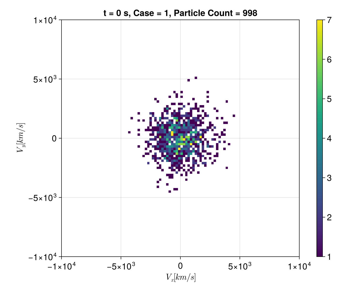

Initial velocity distribution.

julia

f = plot_dist(sols, t = tspan[2], case = 1, slice = :xy)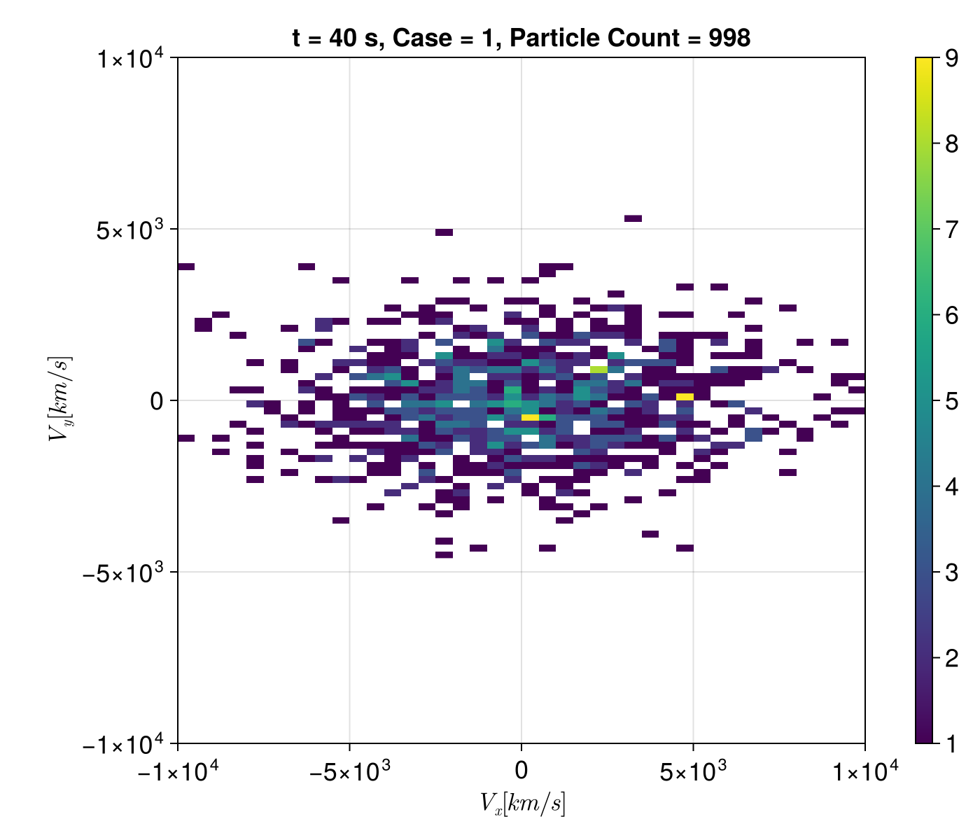

Final velocity distribution

Case 2: B fluctuation core field In this case we use the native Boris pusher for demonstration. The smallest electron gyroperiod in the magnetosheath (B ∼ 20 nT) is about $2 \times 10^{- 3} s$ , and we use a time step $Δ t = 2 \times 10^{- 4} s$ .

julia

const δBfunc = let
    x = range(0.5Rₑ, 1.5Rₑ, length = 10000)
    δB = get_B_perturb(x)
    TP.Field(TP.getinterp(δB, x, 1, 3))
end

dt = 2.0e-4 # [s]
param = prepare(E, Bcase2; species = Electron);
prob = TraceProblem(stateinit, tspan, param; prob_func)
sols = TP.solve(prob; dt, trajectories, isoutofdomain, savestepinterval = 100);

# maximum acceleration ratio particle index
imax = find_max_acceleration_index(sols)

f = plot_multiple(sols[imax])

Trajectory of the most accelerated electron. Note that there are locations where we see a jump in kinetic energy with no electric field peaks; these are artifacts because we only save every 100 steps.

julia

f = plot_dist(sols, t = tspan[1], case = 2, slice = :xy)

Initial velocity distribution.

julia

f = plot_dist(sols, t = tspan[2], case = 2, slice = :xy)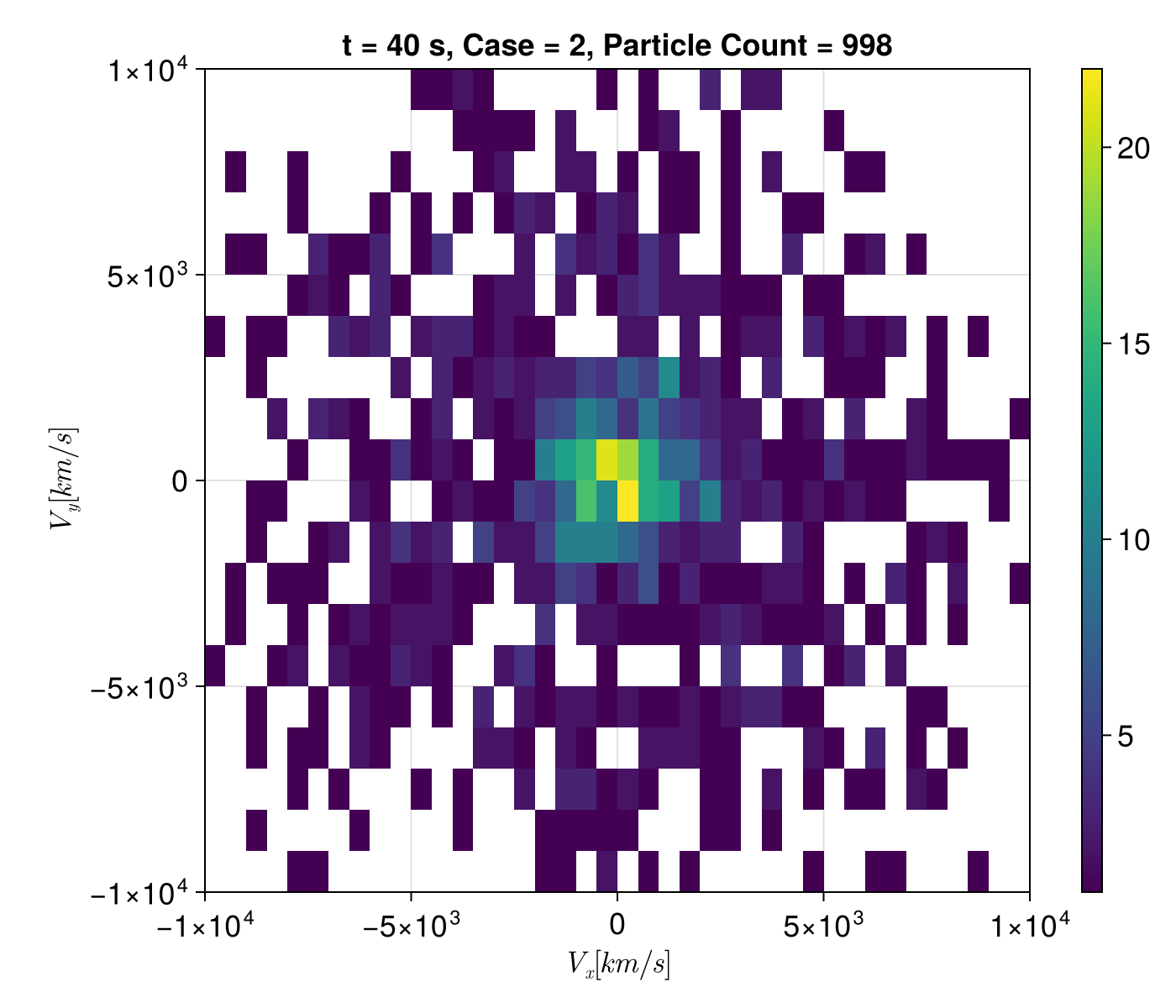

Final velocity distribution

Electron Fermi Acceleration Inside Foreshock Transient Cores ​

Electron Fermi Acceleration Inside Foreshock Transient Cores