Radiation

For an electron undergoing gyromotion in a constant magnetic field, the energy loss is caused by the emission of electromagnetic radiation. The rate of this energy loss (radiated power $P$) depends on whether the electron's speed is relativistic or non-relativistic. This phenomenon is generally divided into two regimes: Cyclotron Radiation (non-relativistic) and Synchrotron Radiation (relativistic).

1. General Formula (Relativistic)

For an electron with charge $e$, mass $m$, and velocity $v$ moving in a magnetic field $B$, the total radiated power $P$ is given by the relativistic generalization of the Larmor formula:

$$P=\frac{e^4{B}^2{\gamma }^2{v}_{\perp }^2}{6\pi {ϵ}_0{m}^2{c}^3}$$

Alternatively, using $\beta =v/c$ and the pitch angle $\alpha$ (where $v_{\perp }=v\sin \alpha$), this is often expressed as:

$$P=\frac{e^4{B}^2{\gamma }^2{\beta }^2{\sin }^2\alpha }{6\pi {ϵ}_0{m}^{2}c}$$

where:

$$\gamma =\frac{1}{\sqrt{1-{\beta }^2}}$$

is the Lorentz factor.

• $${ϵ}_0$$

  is the vacuum permittivity.

• $$c$$

  is the speed of light.

• $$\alpha$$

  is the pitch angle between the velocity vector and the magnetic field vector.

Note on Emission Pattern: In the relativistic regime ($\gamma \gg 1$), the radiation is beamed forward in a narrow cone along the direction of the electron's instantaneous velocity (the "searchlight effect"), which is characteristic of Synchrotron radiation.

1. Non-Relativistic Limit (Cyclotron Radiation)

When the electron speed is much less than the speed of light ($\beta \ll 1$ and $\gamma \approx 1$), the formula simplifies to the classical Cyclotron radiation formula:

$$P\approx \frac{e^4{B}^2{v}_{\perp }^2}{6\pi {ϵ}_0{m}^2{c}^3}$$

Using the Thomson cross-section ${\sigma }_T=\frac{e^4}{6\pi {ϵ}_0^2{m}^2{c}^4}$ and magnetic energy density $U_B=\frac{B^2}{2{\mu }_0}$, this can be written elegantly as:

$$P=2{\sigma }_{T}c{U}_B{\beta }_{\perp }^2$$

1. Energy Loss Per Turn

In accelerator physics, it is often useful to know the energy lost per complete revolution. For a highly relativistic electron ($\beta \approx 1$) moving in a circle of radius $\rho$ (where $\rho \approx \frac{E}{ecB}$), the energy loss per turn $\delta E$ is:

$$\delta E=\oint Pdt=\frac{e^2}{3{ϵ}_0\rho }{\gamma }^4$$

This ${\gamma }^4$ dependence explains why circular electron accelerators (synchrotrons) become inefficient at very high energies—doubling the energy increases the radiative loss by a factor of 16.

1. Cooling Time

The electron will lose energy over time, causing its orbit to decay. The characteristic cooling time $\tau$ (the time scale over which the electron loses a significant fraction of its energy) is:

$$\tau \approx \frac{E}{P}\approx \frac{3m^3{c}^5}{2e^4{B}^2\gamma }$$

In the non-relativistic limit, this simplifies to $\tau \approx \frac{3m^3{c}^5}{4e^4{B}^2}$ (note the independence from energy in the classical limit).

All the above equations are shown in CGS units.

using TestParticle: qᵢ as e, mₑ, c, ϵ₀
using CairoMakie

Physics Functions

"""
    calc_gamma(β)

Calculate the Lorentz factor γ given β (v/c).
"""
function calc_gamma(β)
   if β >= 1.0
      return Inf
   end
   return 1.0 / sqrt(1.0 - β^2)
end

"""
    radiated_power(B, β, α)

Calculate the instantaneous power radiated by an electron in a magnetic field.
Based on the relativistic generalization of the Larmor formula.

Parameters:
B: Magnetic field strength [Tesla]
β: Normalized velocity (v/c)
α: Pitch angle [radians] (angle between v and B)

Returns:
P     : Radiated Power [Watts]
"""
function radiated_power(B, β, α)
   gamma = calc_gamma(β)

   # Formula: P = (e^4 * B^2 * γ^2 * v_perp^2) / (6 * π * ϵ₀ * m^2 * c^3)
   # Substitute v_perp = v * sin(α) = β * c * sin(α)
   # Result: P = (e^4 * B^2 * γ^2 * β^2 * sin(α)^2) / (6 * π * ϵ₀ * m^2 * c)

   numerator = e^4 * B^2 * gamma^2 * β^2 * sin(α)^2
   denominator = 6 * π * ϵ₀ * (mₑ^2) * c

   return numerator / denominator
end

Main.radiated_power

Visualization

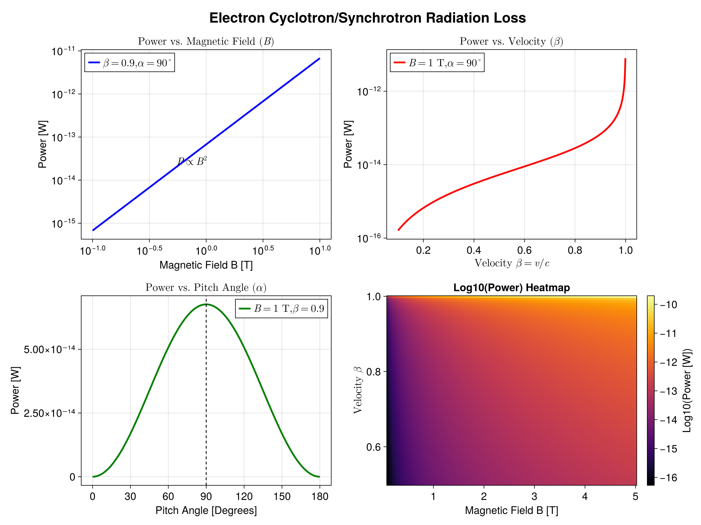
function main()
   fig = Figure(size = (1200, 900), fontsize = 18)

   # --- Plot: Power vs Magnetic Field B ---
   # Fixed parameters
   beta_fixed_1 = 0.9
   alpha_fixed_1 = π / 2 # Perpendicular

   B_range = range(0.1, 10.0, length = 200) # 0.1 T to 10 T
   P_B = radiated_power.(B_range, beta_fixed_1, alpha_fixed_1)

   ax1 = Axis(fig[1, 1],
      title = L"Power vs. Magnetic Field ($B$)",
      xlabel = "Magnetic Field B [T]",
      ylabel = "Power [W]",
      xscale = log10,
      yscale = log10
   )
   lines!(ax1, B_range, P_B, color = :blue, linewidth = 3,
      label = L"\beta = 0.9, \alpha = 90^\circ")
   axislegend(ax1, position = :lt)
   text!(ax1, B_range[10], P_B[10], text = L"P \propto B^2", align = (:left, :bottom))

   # --- Plot: Power vs Velocity (β) ---
   # Fixed parameters
   B_fixed_2 = 1.0 # 1 Tesla
   alpha_fixed_2 = π / 2

   # Range close to 1 to show relativistic effects
   beta_range = range(0.1, 0.999, length = 500)
   P_beta = radiated_power.(B_fixed_2, beta_range, alpha_fixed_2)

   ax2 = Axis(fig[1, 2],
      title = L"Power vs. Velocity ($\beta$)",
      xlabel = L"Velocity $\beta = v/c$",
      ylabel = "Power [W]",
      yscale = log10
   )
   lines!(ax2, beta_range, P_beta, color = :red, linewidth = 3,
      label = L"B = 1\text{ T}, \alpha = 90^\circ")
   axislegend(ax2, position = :lt)

   # --- Plot: Power vs Pitch Angle (α) ---
   # Fixed parameters
   B_fixed_3 = 1.0
   beta_fixed_3 = 0.9

   alpha_range = range(0, π, length = 360)
   alpha_deg = rad2deg.(alpha_range)
   P_alpha = radiated_power.(B_fixed_3, beta_fixed_3, alpha_range)

   ax3 = Axis(fig[2, 1],
      title = L"Power vs. Pitch Angle ($\alpha$)",
      xlabel = "Pitch Angle [Degrees]",
      ylabel = "Power [W]",
      xticks = 0:30:180
   )
   lines!(ax3, alpha_deg, P_alpha, color = :green,
      linewidth = 3, label = L"B=1\text{ T}, \beta=0.9")
   # Add a visual marker for max power
   vlines!(ax3, [90], color = :black, linestyle = :dash)
   axislegend(ax3)

   # --- Plot: Heatmap (Log Power) vs B and β ---
   # Here we vary both B and β
   B_hm = range(0.1, 5.0, length = 100)
   beta_hm = range(0.5, 0.999, length = 100)

   # Calculate matrix
   P_matrix = log10.(radiated_power.(B_hm, beta_hm', π / 2))

   ax4 = Axis(fig[2, 2],
      title = "Log10(Power) Heatmap",
      xlabel = "Magnetic Field B [T]",
      ylabel = L"Velocity $\beta$"
   )
   hm = heatmap!(ax4, B_hm, beta_hm, P_matrix, colormap = :inferno)
   Colorbar(fig[2, 3], hm, label = "Log10(Power [W])")

   Label(fig[0, :], "Electron Cyclotron/Synchrotron Radiation Loss",
      fontsize = 24, font = :bold)

   fig
end

main (generic function with 1 method)

Run the visualization

f = main()

We need to consider radiation effects when the timescale of energy loss (the "cooling time") becomes comparable to or shorter than the characteristic timescale of our system (e.g., confinement time, acceleration time, or simulation duration).

$$\tau \approx \frac{E}{P}=\frac{6\pi {ϵ}_0{m}^3{c}^3}{e^4{B}^2\gamma }=\frac{5.2}{B^2\gamma }\text{ seconds (where B is in Tesla)}$$

• Weak Fields / Low Energy: If $B=1\text{ T}$ and the electron is non-relativistic

($\gamma \approx 1$), $\tau \approx 5$ seconds. You can safely ignore radiation.

• Strong Fields / High Energy: If $B=5\text{ T}$ and you have a 1 GeV electron

($\gamma \approx 2000$), then $\tau \approx 2.5$ milliseconds.