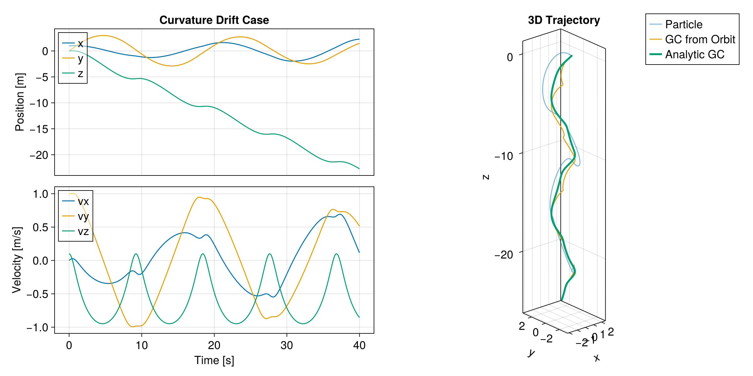
Curvature Drift

This example demonstrates a single proton motion under a non-uniform curved B field with ∇B ⊥ B. It is more complex than the simpler ExB Drift. More theoretical details can be found in Curvature Drift, and Fundamentals of Plasma Physics by Paul Bellan.

using TestParticle, OrdinaryDiffEq, StaticArrays
using LinearAlgebra: norm
using CairoMakie

Plotting Function

We define a function to visualize the results.

function plot_drift_case(sol, sol_gc, title)
    fig = Figure(size = (1200, 600), fontsize = 18)

    # 1. Left Column: Time Series
    gl_left = fig[1, 1] = GridLayout()
    ax_pos = Axis(gl_left[1, 1], ylabel = "Position [m]", title = title)
    lines!(ax_pos, sol, idxs = (0, 1), label = "x")
    lines!(ax_pos, sol, idxs = (0, 2), label = "y")
    lines!(ax_pos, sol, idxs = (0, 3), label = "z")
    axislegend(ax_pos, position = :lt, framevisible = true, backgroundcolor = (:white, 0.5))
    hidexdecorations!(ax_pos, grid = false)

    ax_vel = Axis(gl_left[2, 1], xlabel = "Time [s]", ylabel = "Velocity [m/s]")
    lines!(ax_vel, sol, idxs = (0, 4), label = "vx")
    lines!(ax_vel, sol, idxs = (0, 5), label = "vy")
    lines!(ax_vel, sol, idxs = (0, 6), label = "vz")
    axislegend(ax_vel, position = :lt, framevisible = true, backgroundcolor = (:white, 0.5))

    linkxaxes!(ax_pos, ax_vel)

    # 2. Right Column: 3D Trajectory
    ax_3d = Axis3(
        fig[1, 2];
        title = "3D Trajectory", xlabel = "x", ylabel = "y", zlabel = "z", aspect = :data
    )

    gc = get_gc_func(sol_gc.prob.p)
    gc_plot(x, y, z, vx, vy, vz) = (gc(SA[x, y, z, vx, vy, vz])...,)

    lines!(
        ax_3d, sol;
        idxs = (1, 2, 3),
        color = Makie.wong_colors()[1],
        alpha = 0.5,
        label = "Particle"
    )
    lines!(
        ax_3d, sol;
        idxs = (gc_plot, 1, 2, 3, 4, 5, 6),
        color = Makie.wong_colors()[2],
        label = "GC from Orbit"
    )
    lines!(
        ax_3d, sol_gc;
        idxs = (1, 2, 3),
        color = Makie.wong_colors()[3],
        linewidth = 3,
        label = "Analytic GC"
    )
    axislegend(ax_3d, framevisible = true, backgroundcolor = (:white, 0.5))

    return fig
end

plot_drift_case (generic function with 1 method)

Curvature B Field

We use a curved magnetic field and trace a proton.

curved_B(x) = SA[x[2] / norm(x[1:2])^2, -x[1] / norm(x[1:2])^2, 0.0] * 1.0e-8
zero_E(x) = SA[0.0, 0.0, 0.0]

# Initial conditions
stateinit = let x0 = [1.0, 0.0, 0.0], v0 = [0.0, 1.0, 0.1]
    [x0..., v0...]
end
# Time span
tspan = (0, 40)
# Trace particle
param = prepare(zero_E, curved_B, species = Proton)
prob = ODEProblem(trace!, stateinit, tspan, param)
sol = solve(prob, Vern9())
# Functions for obtaining the guiding center from actual trajectory
gc = param |> get_gc_func
gc_x0 = gc(stateinit) |> Vector
prob_gc = ODEProblem(trace_gc_drifts!, gc_x0, tspan, (param..., sol))
sol_gc = solve(prob_gc, Vern7(); save_idxs = [1, 2, 3])

fig = plot_drift_case(sol, sol_gc, "Curvature Drift Case")