Adaptive Solver Accuracy
This example compares the accuracy and energy conservation of solvers that use changing time steps: the native AdaptiveBoris solver and the adaptive ODE solvers Tsit5 and Vern6.
Unlike the fixed-step tests in Solver Accuracy Analysis and Energy Conservation, these tests exercise the adaptive time-stepping machinery where dt changes during the simulation — e.g., the Boris velocity resync at dt transitions and the ODE error controllers.
Three cases are presented: 2. Magnetic Mirror — energy conservation with spatially varying |B|.
Constant E + B — accuracy convergence sweeping safety η (dt / T_gyro).
ExB Drift — long-term energy conservation.
using Printf
using TestParticle
import TestParticle as TP
using OrdinaryDiffEq
using StaticArrays
using LinearAlgebra: norm, ×, ⋅
using CairoMakie

const q = 1.0
const m = 1.0
const B₀ = 1.0
const Ω = q * B₀ / m
const T_gyro = 2π / Ω

function energy_error(sol, E_ref_func)
    errs = Float64[]
    for (t, u) in zip(sol.t, sol.u)
        v_mag2 = u[4]^2 + u[5]^2 + u[6]^2
        E_kin = 0.5 * m * v_mag2
        E_ref = E_ref_func(t, u)
        push!(
            errs,
            abs(E_kin - E_ref) / (abs(E_ref) + 1.0e-16),
        )
    end
    return errs
end

function plot_table(results)
    io = IOBuffer()
    println(io, "| Solver | Max Rel. Error |")
    println(io, "| :--- | :--- |")
    for (name, err) in results
        println(io, "| $name | $(@sprintf("%.1e", err)) |")
    end
    return Markdown.parse(String(take!(io)))
end
plot_table (generic function with 1 method)Case 1: Magnetic Mirror — Energy Conservation
The magnetic mirror field is ideal for testing adaptive Boris: the spatially varying |B| causes genuine dt changes as the particle moves between weak-field and strong-field regions. Since E = 0, total kinetic energy should be exactly conserved.
The field is divergence-free in cylindrical symmetry:
function mirror_B(x)
    α = 0.1
    Bz = B₀ * (1 + α * x[3]^2)
    Bx = -B₀ * α * x[1] * x[3]
    By = -B₀ * α * x[2] * x[3]
    return SA[Bx, By, Bz]
end

param1 = prepare(ZeroField(), mirror_B; q, m)
x0_1 = [0.1, 0.0, 0.0]
v0_1 = [0.5, 0.5, 1.0]
u0_1 = [x0_1..., v0_1...]
tspan1 = (0.0, 200.0)
E_init = 0.5 * m * norm(v0_1)^2

prob_tp1 = TraceProblem(u0_1, tspan1, param1)
prob_ode1 = ODEProblem(trace_normalized!, u0_1, tspan1, param1)

adaptive_solvers_1 = [
    (
        "AdaptiveBoris (η=1/16)",
        AdaptiveBoris(; safety = 1 / 16),
    ),
    (
        "AdaptiveBoris (η=1/8)",
        AdaptiveBoris(; safety = 1 / 8),
    ),
    (
        "AdaptiveBoris (η=1/4)",
        AdaptiveBoris(; safety = 1 / 4),
    ),
]

ode_solvers_1 = [
    ("Tsit5 (default tol)", Tsit5(), Dict()),
    (
        "Tsit5 (tight tol)", Tsit5(),
        Dict(:abstol => 1.0e-10, :reltol => 1.0e-10),
    ),
    ("Vern6 (default tol)", Vern6(), Dict()),
    (
        "Vern6 (tight tol)", Vern6(),
        Dict(:abstol => 1.0e-10, :reltol => 1.0e-10),
    ),
]

f1 = Figure(; size = (1200, 500), fontsize = 20)

ax1a = Axis(
    f1[1, 1];
    yscale = log10,
    xlabel = "Time [Gyroperiod]",
    ylabel = "Rel. Energy Error",
    title = "Magnetic Mirror: Energy Error",
    yminorticksvisible = true,
    yminorticks = IntervalsBetween(9),
)
ylims!(ax1a, 1.0e-16, 1.0)

ax1b = Axis(
    f1[1, 2];
    xlabel = "Time [Gyroperiod]",
    ylabel = L"\Delta t / T_\mathrm{gyro}",
    title = "AdaptiveBoris: Time Step History",
)

for (i, (name, alg)) in enumerate(adaptive_solvers_1)
    sol = TP.solve(prob_tp1, alg).u[1]
    errs = energy_error(sol, (t, u) -> E_init)
    lines!(
        ax1a, sol.t ./ T_gyro, errs;
        label = name,
        color = i, colormap = :tab10, colorrange = (1, 10),
    )
    dts = diff(sol.t)
    lines!(
        ax1b,
        sol.t[1:(end - 1)] ./ T_gyro,
        dts ./ T_gyro;
        label = name,
        color = i, colormap = :tab10, colorrange = (1, 10),
    )
end

n_boris = length(adaptive_solvers_1)
for (i, (name, alg, kwargs)) in enumerate(ode_solvers_1)
    sol = solve(prob_ode1, alg; dense = false, kwargs...)
    errs = energy_error(sol, (t, u) -> E_init)
    lines!(
        ax1a, sol.t ./ T_gyro, errs;
        label = name,
        color = n_boris + i,
        colormap = :tab10, colorrange = (1, 10),
    )
    dts = diff(sol.t)
    lines!(
        ax1b,
        sol.t[1:(end - 1)] ./ T_gyro,
        dts ./ T_gyro;
        label = name,
        color = n_boris + i, colormap = :tab10, colorrange = (1, 10),
    )
end

f1[1, 3] = Legend(f1, ax1a; framevisible = false)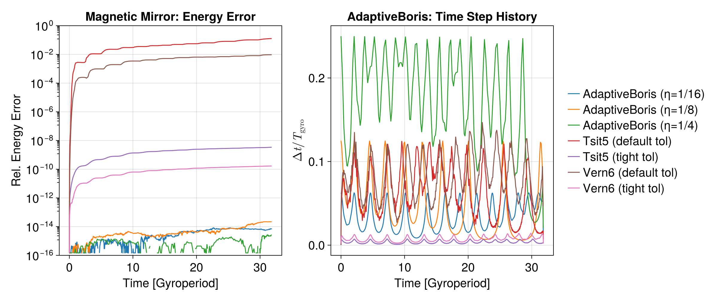
Summary
results1 = Tuple{String, Float64}[]

for (name, alg) in adaptive_solvers_1
    sol = TP.solve(prob_tp1, alg).u[1]
    errs = energy_error(sol, (t, u) -> E_init)
    push!(results1, (name, maximum(errs)))
end
for (name, alg, kwargs) in ode_solvers_1
    sol = solve(prob_ode1, alg; dense = false, kwargs...)
    errs = energy_error(sol, (t, u) -> E_init)
    push!(results1, (name, maximum(errs)))
end| Solver | Max Rel. Error |
|---|---|
| AdaptiveBoris (η=1/16) | 8.3e-15 |
| AdaptiveBoris (η=1/8) | 2.2e-14 |
| AdaptiveBoris (η=1/4) | 2.7e-15 |
| Tsit5 (default tol) | 1.3e-01 |
| Tsit5 (tight tol) | 3.4e-09 |
| Vern6 (default tol) | 9.5e-03 |
| Vern6 (tight tol) | 1.7e-10 |
Case 2: Constant E + B — Accuracy Convergence
With E = [0, 0.5, 0.1] and B = [0, 0, 1], an exact velocity solution exists (Section 6, Zenitani & Kato 2025). We sweep the safety parameter η (representing dt / T_gyro) for AdaptiveBoris and the tolerance for the ODE solvers, then plot maximum velocity error vs. number of time steps (computational cost).
B_func2(x, t) = SA[0.0, 0.0, 1.0]
E_func2(x, t) = SA[0.0, 0.5, 0.1]

const E_vec = SA[0.0, 0.5, 0.1]
const B_vec = SA[0.0, 0.0, 1.0]

function exact_velocity(t)
    vD = (E_vec × B_vec) / (B₀^2)
    E_par = (E_vec ⋅ (B_vec / B₀)) * (B_vec / B₀)
    b̂ = B_vec / B₀
    v_perp = -vD * cos(Ω * t) -
        (vD × b̂) * sin(Ω * t) + vD
    v_para = (q * E_par / m) * t
    return v_perp + v_para
end

t_end2 = 6 * T_gyro
tspan2 = (0.0, t_end2)
u0_2 = [0.0, 0.0, 0.0, 0.0, 0.0, 0.0]
param2 = prepare(E_func2, B_func2; q, m)
prob_tp2 = TraceProblem(u0_2, tspan2, param2)
prob_ode2 = ODEProblem(trace_normalized!, u0_2, tspan2, param2)

function max_velocity_error(sol)
    max_err = 0.0
    for (t, u) in zip(sol.t, sol.u)
        v_num = SA[u[4], u[5], u[6]]
        v_ana = exact_velocity(t)
        max_err = max(max_err, norm(v_num - v_ana))
    end
    return max_err
end

safety_values = range(0.01, 0.2, length = 10)
tol_values = logrange(1.0e-12, 1.0e-2, length = 10)

boris_steps = Int[]
boris_errors = Float64[]

for s in safety_values
    alg = AdaptiveBoris(; safety = s)
    sol = TP.solve(prob_tp2, alg).u[1]
    push!(boris_steps, length(sol.t))
    push!(boris_errors, max_velocity_error(sol))
end

ode_results_2 = Dict{
    String, Tuple{Vector{Int}, Vector{Float64}},
}()

for (name, alg) in [("Tsit5", Tsit5()), ("Vern6", Vern6())]
    steps_vec = Int[]
    err_vec = Float64[]
    for tol in tol_values
        sol = solve(
            prob_ode2, alg;
            abstol = tol, reltol = tol, dense = false,
        )
        push!(steps_vec, length(sol.t))
        push!(err_vec, max_velocity_error(sol))
    end
    ode_results_2[name] = (steps_vec, err_vec)
end
Visualization
f2 = Figure(; size = (700, 500), fontsize = 20)

ax2 = Axis(
    f2[1, 1];
    xscale = log10,
    yscale = log10,
    xlabel = "Number of Time Steps",
    ylabel = "Max Velocity Error",
    title = "Accuracy vs. Cost (Adaptive Solvers)",
    xminorticksvisible = true,
    yminorticksvisible = true,
    xminorticks = IntervalsBetween(9),
    yminorticks = IntervalsBetween(9),
)

scatterlines!(
    ax2, boris_steps, boris_errors;
    label = "AdaptiveBoris",
    marker = :circle, linewidth = 2,
)

for (name, (steps_vec, err_vec)) in ode_results_2
    scatterlines!(
        ax2, steps_vec, err_vec;
        label = "$name (adaptive)",
        marker = :cross, linewidth = 2,
    )
end

axislegend(ax2; position = :rt, framevisible = false)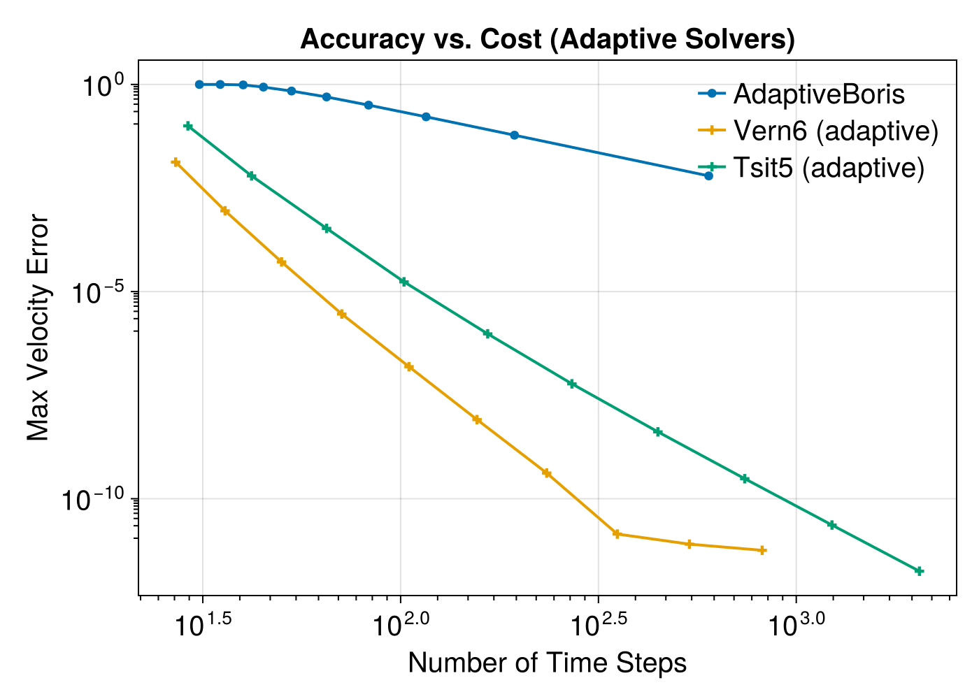
Case 3: ExB Drift — Long-term Energy Conservation
Using the same E and B as Case 2, the analytical kinetic energy gain is known exactly. We run for 200 gyroperiods to expose long-term drift.
const Ey_val = 0.5
const Ez_val = 0.1

function E_ref3(t, u)
    vx = (Ey_val / B₀) * (1 - cos(Ω * t))
    vy = (Ey_val / B₀) * sin(Ω * t)
    vz = (q * Ez_val / m) * t
    return 0.5 * m * (vx^2 + vy^2 + vz^2)
end

t_end3 = 200 * T_gyro
tspan3 = (0.0, t_end3)
param3 = prepare(E_func2, B_func2; q, m)
prob_tp3 = TraceProblem(u0_2, tspan3, param3)
prob_ode3 = ODEProblem(trace_normalized!, u0_2, tspan3, param3)

adaptive_solvers_3 = [
    (
        "AdaptiveBoris (η=0.1)",
        AdaptiveBoris(; safety = 0.1),
    ),
    (
        "AdaptiveBoris (η=0.2)",
        AdaptiveBoris(; safety = 0.2),
    ),
]

ode_solvers_3 = [
    ("Tsit5 (default tol)", Tsit5(), Dict()),
    (
        "Tsit5 (tight tol)", Tsit5(),
        Dict(:abstol => 1.0e-10, :reltol => 1.0e-10),
    ),
    ("Vern6 (default tol)", Vern6(), Dict()),
    (
        "Vern6 (tight tol)", Vern6(),
        Dict(:abstol => 1.0e-10, :reltol => 1.0e-10),
    ),
]

f3 = Figure(; size = (900, 500), fontsize = 20)
ax3 = Axis(
    f3[1, 1];
    yscale = log10,
    xlabel = "Time [Gyroperiod]",
    ylabel = L"""Rel. Energy Error
    $|(E - E_\mathrm{ref})/E_\mathrm{ref}|$""",
    title = "ExB Drift: Long-term Energy Error",
    yminorticksvisible = true,
    yminorticks = IntervalsBetween(9),
)
xlims!(ax3, 0.0, 200.0)
ylims!(ax3, 1.0e-16, 1.0)

results3 = Tuple{String, Float64}[]

for (i, (name, alg)) in enumerate(adaptive_solvers_3)
    sol = TP.solve(prob_tp3, alg).u[1]
    errs = energy_error(sol, E_ref3)
    lines!(
        ax3, sol.t ./ T_gyro, errs;
        label = name,
        color = i, colormap = :tab10, colorrange = (1, 10),
    )
    push!(results3, (name, maximum(errs)))
end

n_ab = length(adaptive_solvers_3)
for (i, (name, alg, kwargs)) in enumerate(ode_solvers_3)
    sol = solve(prob_ode3, alg; dense = false, kwargs...)
    errs = energy_error(sol, E_ref3)
    lines!(
        ax3, sol.t ./ T_gyro, errs;
        label = name,
        color = n_ab + i,
        colormap = :tab10, colorrange = (1, 10),
    )
    push!(results3, (name, maximum(errs)))
end

f3[1, 2] = Legend(f3, ax3; framevisible = false)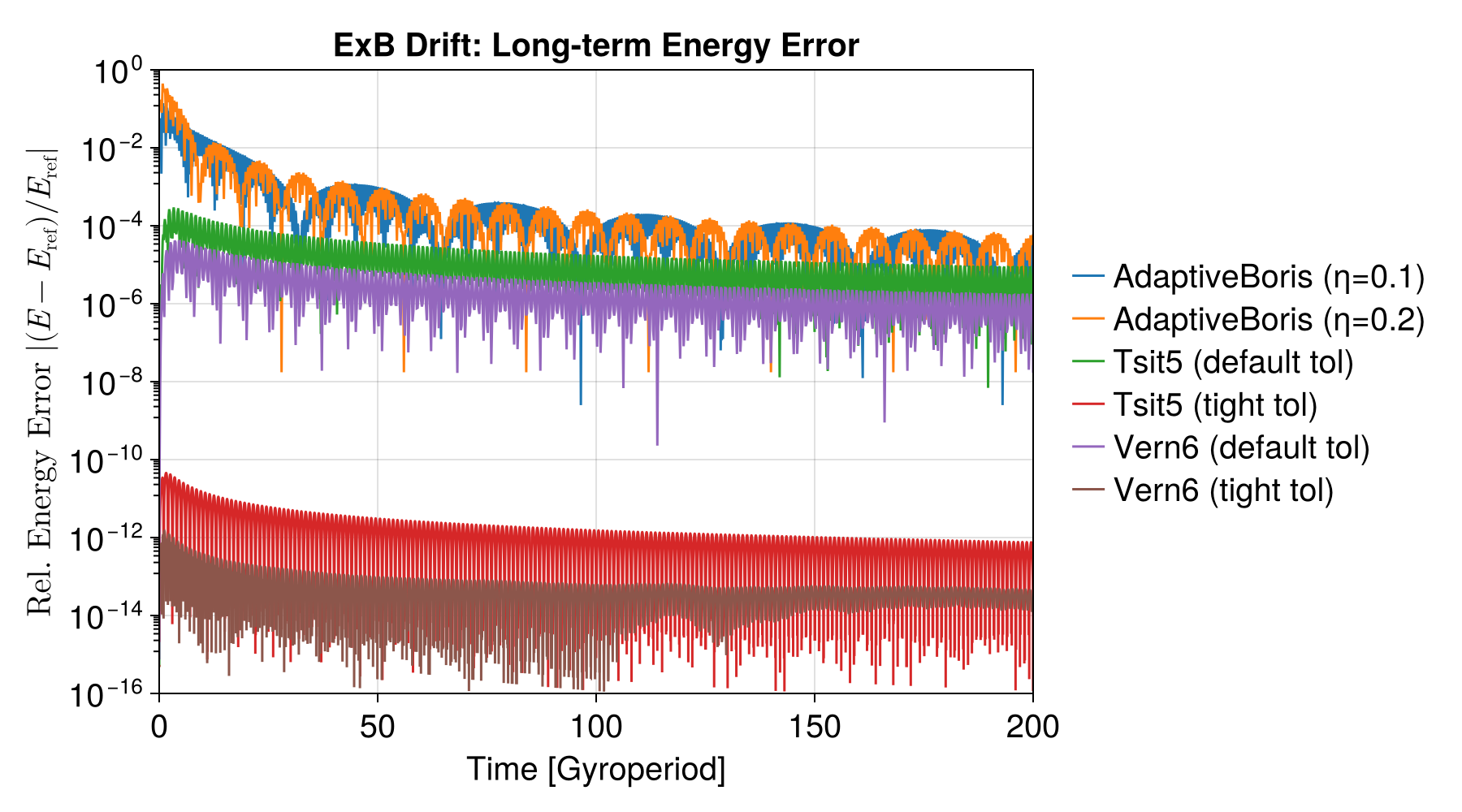
Summary
| Solver | Max Rel. Error |
|---|---|
| AdaptiveBoris (η=0.1) | 1.4e-01 |
| AdaptiveBoris (η=0.2) | 4.4e-01 |
| Tsit5 (default tol) | 3.0e-04 |
| Tsit5 (tight tol) | 4.5e-11 |
| Vern6 (default tol) | 4.2e-05 |
| Vern6 (tight tol) | 1.5e-12 |