Adiabatic Acceleration

This example demonstrates the three fundamental adiabatic acceleration mechanisms using guiding center (GC) tracing:

1. Betatron acceleration: $\mu$ conserved, $\partial B/\partial t>0$ → perpendicular energy gain via $\mu \partial B/\partial t$.

2. Fermi acceleration: curvature and grad-B drifts crossing an electric field → parallel/perpendicular energy exchange.

3. Local $E_{\parallel }$ acceleration: direct acceleration by the parallel electric field component $q{v}_{\parallel }(\mathbf{E}\cdot \hat{\mathbf{b}})$.

The physical setup uses a mirror-confined, sheared, time-dependent magnetic field with a constant electric field, inducing all three mechanisms simultaneously. The energy gain is decomposed using the GC work rate formulas from Northrop (1963).

References:

• Key Notes: Particle Acceleration

• Northrop, T. G. (1963). The Adiabatic Motion of Charged Particles.

using TestParticle, OrdinaryDiffEq, StaticArrays
import TestParticle as TP
using LinearAlgebra: norm
using CairoMakie

Physical Setup

The magnetic field is a sheared, divergence-free field with a $\tanh$ profile that creates a magnetic mirror:

$$\mathbf{B}(\mathbf{x},t)=B_0(t)\left[\begin{array}{c}\alpha L\tanh (z/L)+\delta \\ 0\\ 1\end{array}\right],B_0(t)=B_{00}(1+\beta t).$$

Near $z=0$, $\tanh (z/L)\approx z/L$, giving $B_x\approx \alpha z+\delta$. The $\tanh$ growth increases $|\mathbf{B}|$ away from the midplane, forming a magnetic mirror that confines the particle near $z=0$ where field-line curvature and gradient are strongest. This field has:

• Curvature $\mathit{\kappa }\ne 0$ (strongest near $z=0$)

• Gradient $\mathrm{\nabla }B\ne 0$ (from the $z$-dependence of $B_x$, non-zero everywhere due to $\delta$)

• Time dependence $\partial B/\partial t\ne 0$ (from the $B_0(t)$ ramp)

The electric field is constant:

$$\mathbf{E}=\left[\begin{array}{c}0\\ E_{\perp }\\ E_{\parallel }\end{array}\right].$$

$E_{\perp }$ couples to the curvature and grad-B drifts (Fermi mechanism), while $E_{\parallel }$ directly accelerates particles along the field line.

Adiabaticity Check

The adiabatic parameter $ϵ={\rho }_L/L_B$ where ${\rho }_L$ is the gyroradius and $L_B=|\mathrm{\nabla }B{|}^{-1}B$ is the field gradient scale at $z=0$:

$${\rho }_L=\frac{m{v}_{\perp }}{|q|B}\approx 2.6\mathrm{m},L_B\approx \frac{1+{\delta }^2}{\alpha \delta }=\frac{2}{0.2\times 1.0}=10\mathrm{m},ϵ\approx 0.26.$$

The adiabatic parameter is $\lesssim 0.3$ throughout, keeping the GC description adequate for this demonstration.

# --- Parameters (SI units) ---
const B₀₀ = 1.0e-4    # baseline field strength [T]
const α = 0.2         # gradient strength at z = 0 [m⁻¹]
const L_z = 200.0     # Bx saturation scale length [m]; creates a magnetic mirror
const δ = 1.0         # B_x offset; breaks z-symmetry
const β = 0.1         # compression rate [1/s]
const E_perp = 1.0e-4 # perpendicular E field [V/m]
const E_par = 2.0e-4  # parallel E field base [V/m]
const L_E = 30.0      # E-field gradient scale length [m]; breaks bounce symmetry

const eV = TP.eV  # electron volt [J]

# Time-dependent B₀
B₀(t) = B₀₀ * (1 + β * t)

# Mirror-confined sheared magnetic field: Bx(z) = α L tanh(z/L) + δ, ∇·B = 0
function shear_B(x, t = 0.0)
    B0t = B₀(t)
    return SA[(α * L_z * tanh(x[3] / L_z) + δ) * B0t, 0.0, B0t]
end

# Constant electric field with both perp and parallel components.
# The z-dependent E∥ breaks the mirror bounce symmetry so that net
# E∥ work accumulates rather than canceling out.
function const_E(x, t = 0.0)
    return SA[0.0, E_perp, E_par * (1.0 + x[3] / L_E)]
end

# --- Species: Proton ---
const species = Proton

# --- Initial Conditions ---
x0 = [0.1, 0.0, 0.0]
v_mag = 5.0e4               # 50 km/s, non-relativistic

# At z = 0, B ∝ (δ, 0, 1) = (1, 0, 1).  Velocity entirely in the x-direction
# gives a 45° pitch angle: v · b̂ = v_mag/√2, |v⟂| = v_mag/√2.
v0 = [v_mag, 0.0, 0.0]

const stateinit = [x0..., v0...]
const tspan = (0.0, 0.799015832364488)

# Report adiabatic parameter
q_p, m_p = species.q, species.m
B_init = norm(shear_B(x0))
b̂_init = shear_B(x0) ./ B_init
vpar_init = sum(v0 .* b̂_init)
vperp_init = norm(v0 .- vpar_init .* b̂_init)
ρ_L = m_p * vperp_init / (abs(q_p) * B_init)
L_B = (1 + δ^2) / (α * δ)  # |∇B| = B₀ αδ/√(1+δ²), B = B₀√(1+δ²) at z=0
println(
    "Adiabatic parameter ε = ρ_L / L_B = ", round(ρ_L, digits = 1),
    " / ", round(L_B, digits = 1), " = ", round(ρ_L / L_B, digits = 2)
)

Adiabatic parameter ε = ρ_L / L_B = 2.6 / 10.0 = 0.26

GC Tracing

We compute the initial GC state and trace the GC equations.

stateinit_gc, param_gc = prepare_gc(
    stateinit, const_E, shear_B; species
)
q, q2m, μ, Efunc, Bfunc = param_gc
m = q / q2m

println(
    "Initial GC: X = ", round.(stateinit_gc[1:3], digits = 3),
    ", v∥ = ", round(stateinit_gc[4], digits = 0), " m/s"
)
println("Magnetic moment μ = ", μ, " J/T")
println(
    "Initial kinetic energy = ", round(
        0.5 * m * stateinit_gc[4]^2 + μ *
            norm(Bfunc(SA[stateinit_gc[1], stateinit_gc[2], stateinit_gc[3]], 0.0)) / eV,
        digits = 1
    ), " eV"
)

prob_gc = ODEProblem(trace_gc!, stateinit_gc, tspan, param_gc)
sol_gc = solve(prob_gc, Vern9())
println("GC solver steps: ", length(sol_gc.t))

Initial GC: X = [0.1, -2.61, 0.0], v∥ = 35355.0 m/s
Magnetic moment μ = 7.391718732059811e-15 J/T
Initial kinetic energy = 6.5 eV
GC solver steps: 2054

Energy Decomposition

The GC work rates (Northrop 1963) decompose $dK/dt$ into:

Term	Formula	Physics
$P_{\parallel }$	$q{v}_{\parallel }(\mathbf{E}\cdot \hat{\mathbf{b}})$	Direct E∥ acceleration
$P_{\mathrm{Fermi}}$	$\frac{m{v}_{\parallel }^2}{B}(\hat{\mathbf{b}}\times \mathit{\kappa })\cdot \mathbf{E}$	Curvature drift × E
$P_{\mathrm{grad}}$	$\frac{\mu }{B}(\hat{\mathbf{b}}\times \mathrm{\nabla }B)\cdot \mathbf{E}$	Grad-B drift × E
$P_{\mathrm{betatron}}$	$\mu \frac{\partial B}{\partial t}$	μ conservation in ∂B/∂t

# Compute work rates and kinetic energy along the GC trajectory
function energy_decomposition(sol, param_gc)
    q, q2m, μ, _, Bfunc = param_gc
    m = q / q2m
    ts = sol.t
    n = length(ts)
    P_arr = zeros(n, 4)  # columns: par, fermi, grad, beta
    K_gc = zeros(n)
    B_along = zeros(n)

    for (i, t) in enumerate(ts)
        xu = sol.u[i]
        X = SA[xu[1], xu[2], xu[3]]
        Bmag_val = norm(Bfunc(X, t))
        B_along[i] = Bmag_val
        K_gc[i] = 0.5 * m * xu[4]^2 + μ * Bmag_val
        wr = TP.get_work_rates_gc(xu, param_gc, t)
        P_arr[i, 1] = wr[1]  # P_par
        P_arr[i, 2] = wr[2]  # P_fermi
        P_arr[i, 3] = wr[3]  # P_grad
        P_arr[i, 4] = wr[4]  # P_betatron
    end

    return P_arr, K_gc, B_along
end

ts = sol_gc.t
n = length(ts)
P_arr, K_gc, B_along = energy_decomposition(sol_gc, param_gc)

# Cumulative work (trapezoidal integration)
function cumtrapz(t, y)
    @assert length(t) == length(y) "Dimension mismatch between t and y"
    out = similar(y, eltype(y), length(t))
    out[1] = zero(eltype(y))
    for i in 2:length(t)
        out[i] = out[i - 1] + 0.5 * (y[i] + y[i - 1]) * (t[i] - t[i - 1])
    end
    return out
end

W_par = cumtrapz(ts, @view P_arr[:, 1])
W_fermi = cumtrapz(ts, @view P_arr[:, 2])
W_grad = cumtrapz(ts, @view P_arr[:, 3])
W_beta = cumtrapz(ts, @view P_arr[:, 4])
W_total = W_par .+ W_fermi .+ W_grad .+ W_beta

# Actual energy change
ΔK_gc = K_gc .- K_gc[1]

# Convert to eV for display
K_gc_eV = K_gc ./ eV
ΔK_gc_eV = ΔK_gc ./ eV
W_par_eV = W_par ./ eV
W_fermi_eV = W_fermi ./ eV
W_grad_eV = W_grad ./ eV
W_beta_eV = W_beta ./ eV
W_total_eV = W_total ./ eV
P_arr_eV = P_arr ./ eV

Quantity	ΔEnergy (eV)
ΔK (GC)	1.07e+00
Σ Work (GC)	8.81e-01
Betatron	8.14e-01
Fermi	2.97e-01
Grad-B	-2.31e-01
E∥ (parallel)	6.12e-04

Visualization

# --- Figure 1: Trajectory and Energy Overview ---
f1 = Figure(size = (1100, 700), fontsize = 14)

ax1 = Axis3(
    f1[1:2, 1],
    title = "GC Trajectory (mirror-confined, time-dependent B)",
    xlabel = "x [m]", ylabel = "y [m]", zlabel = "z [m]",
    aspect = :data,
)
lines!(
    ax1, sol_gc, idxs = (1, 2, 3), color = :steelblue, linewidth = 2,
    label = "Guiding Center"
)
scatter!(
    ax1, [sol_gc.u[1][1]], [sol_gc.u[1][2]], [sol_gc.u[1][3]],
    color = :green, markersize = 12, label = "Start"
)
scatter!(
    ax1, [sol_gc.u[end][1]], [sol_gc.u[end][2]], [sol_gc.u[end][3]],
    color = :red, markersize = 12, label = "End"
)
axislegend(ax1; position = :rt)

# |B| along trajectory
ax2 = Axis(
    f1[1, 2],
    title = "|B| Along GC Trajectory",
    xlabel = "Time [s]", ylabel = "|B| [T]",
)
lines!(ax2, ts, B_along, color = :steelblue, linewidth = 2)

# Kinetic energy
ax3 = Axis(
    f1[2, 2],
    title = "Kinetic Energy (K = ½mv∥² + μB)",
    xlabel = "Time [s]", ylabel = "K [eV]",
)
lines!(ax3, ts, K_gc_eV, color = :steelblue, linewidth = 2)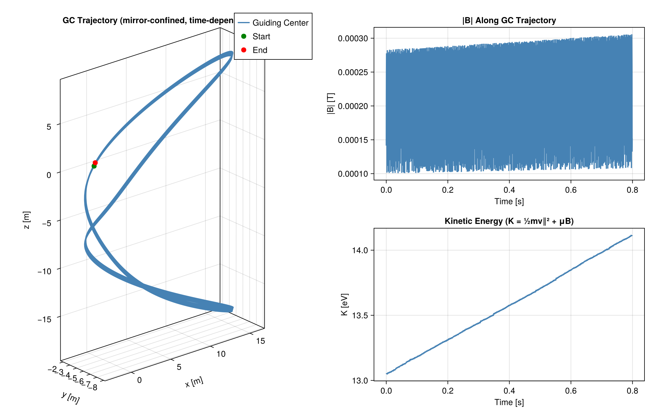

The GC kinetic energy shows a clear secular increase driven by the combined action of all three adiabatic acceleration mechanisms. The magnetic mirror ($\tanh$ profile with $L=200$ m) confines the particle near $z=0$, sustaining curvature and gradient throughout the trajectory so that all work channels accumulate visibly. A small offset between $\mathrm{\Delta }K$ and $\mathrm{\Sigma }$ Work is expected: with $\epsilon ={\rho }_L/L_B\approx 0.26$, the GC work-rate formulas carry $\mathcal{O}(\epsilon )$ truncation error.

# --- Figure 2: Cumulative Work Decomposition ---
f2 = Figure(size = (1100, 800), fontsize = 14)

ax_cum = Axis(
    f2[1, 1],
    title = "Cumulative Work Decomposition",
    xlabel = "Time [s]", ylabel = "Energy Gain [eV]",
)
lines!(
    ax_cum, ts, ΔK_gc_eV, color = :black, linewidth = 2.5,
    label = L"\Delta K\ \mathrm{(actual)}"
)
lines!(
    ax_cum, ts, W_total_eV, color = :black, linestyle = :dash,
    linewidth = 2, label = L"\Sigma\ \mathrm{Work\ rates}"
)
lines!(
    ax_cum, ts, W_beta_eV, color = :coral, linewidth = 2,
    label = L"\mathrm{Betatron}\ (\mu\,\partial B/\partial t)"
)
lines!(
    ax_cum, ts, W_fermi_eV, color = :teal, linewidth = 2,
    label = L"\mathrm{Fermi}\ (\mathbf{v}_c\times\mathbf{E})"
)
lines!(
    ax_cum, ts, W_grad_eV, color = :goldenrod, linewidth = 2,
    label = L"\mathrm{Grad-}B\ \mathrm{drift}\times\mathbf{E}"
)
lines!(
    ax_cum, ts, W_par_eV, color = :purple, linewidth = 2,
    label = L"E_\parallel\ (q v_\parallel\,\mathbf{E}\cdot\hat{\mathbf{b}})"
)
axislegend(ax_cum; position = :lt)

# --- Figure 3: Instantaneous Work Rates ---
ax_inst = Axis(
    f2[2, 1],
    title = "Instantaneous Work Rates",
    xlabel = "Time [s]", ylabel = "Power [eV/s]",
)
@views lines!(
    ax_inst, ts, P_arr_eV[:, 1], color = :purple,
    linewidth = 1.5, label = L"P_\parallel"
)
@views lines!(
    ax_inst, ts, P_arr_eV[:, 2], color = :teal,
    linewidth = 1.5, label = L"P_\mathrm{Fermi}"
)
@views lines!(
    ax_inst, ts, P_arr_eV[:, 3], color = :goldenrod,
    linewidth = 1.5, label = L"P_{\nabla B}"
)
@views lines!(
    ax_inst, ts, P_arr_eV[:, 4], color = :coral,
    linewidth = 1.5, label = L"P_\mathrm{betatron}"
)
axislegend(ax_inst; position = :rt)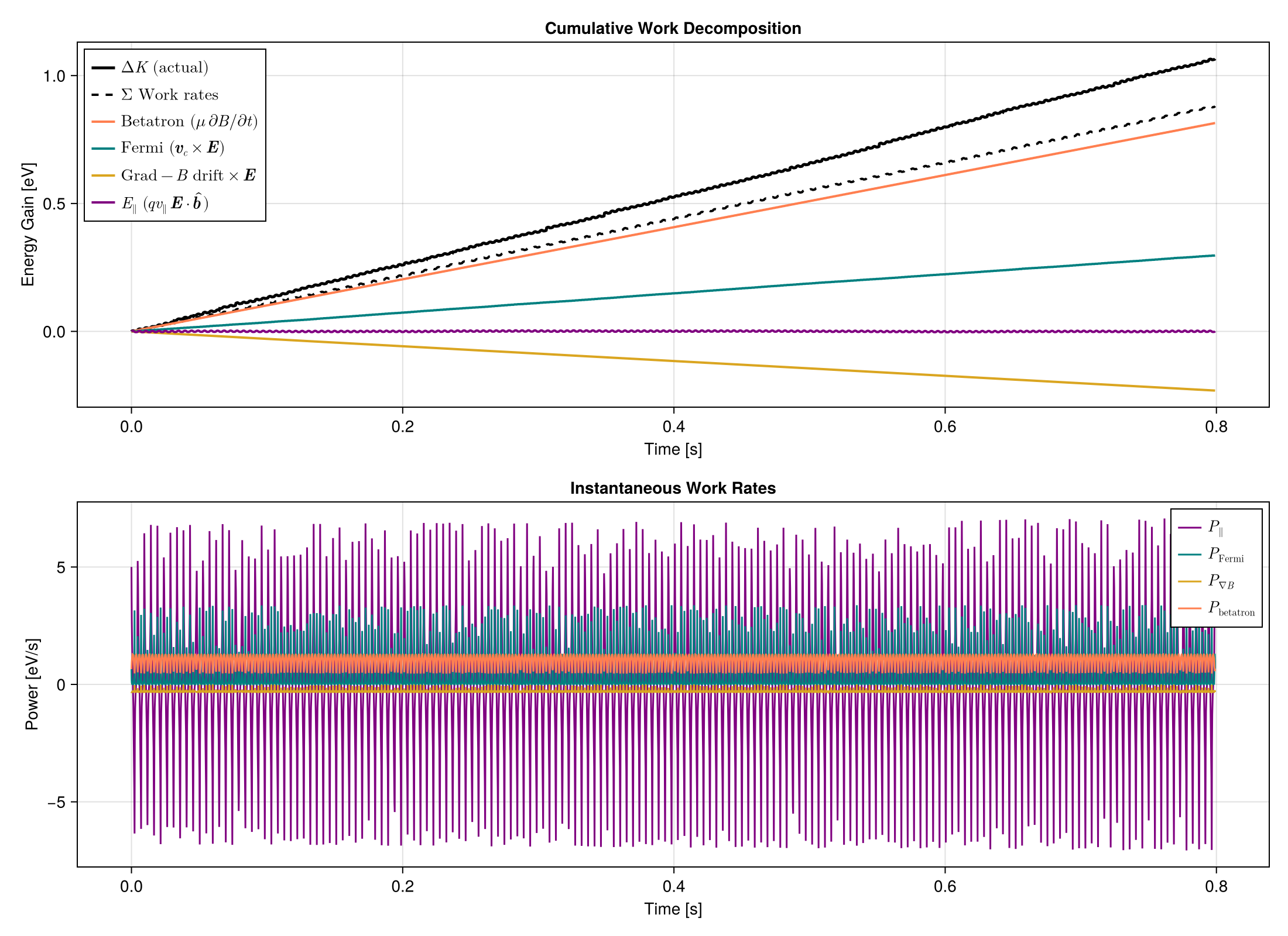

Discussion

The cumulative work decomposition reveals three distinct acceleration channels:

1. Betatron acceleration (coral): $\mu \partial B/\partial t$ provides a steady power input proportional to the field compression rate $\beta$. With the initial velocity at a true ${45}^{\circ }$ pitch angle to $\mathbf{B}$, the magnetic moment is $\mu \approx 7.4\times {10}^{-15}$ J/T, giving $P_{\mathrm{betatron}}\approx 0.65$ eV/s at $z=0$.

2. Fermi + Grad-B drift work (teal + goldenrod): These arise from the curvature and grad-B drifts crossing $E_{\perp }$. The magnetic mirror (mirror ratio $\sim$ 30) confines the particle to $|z|\lesssim 7.5$ m, keeping it within the region where $\mathit{\kappa }$ and $\mathrm{\nabla }B$ are strong. This allows the drift-based work terms to accumulate over many bounce cycles rather than dying out after the first gradient crossing. In this field geometry, the two drift directions partially oppose each other — a known property of magnetostatic equilibria where $\mathrm{\nabla }B$ and $\mathit{\kappa }$ point in opposite directions.

3. Parallel $E_{\parallel }$ (purple): Direct acceleration along $\hat{\mathbf{b}}$ by the parallel electric field. In a uniform $E_{\parallel }$, the mirror bounce causes $v_{\parallel }$ to oscillate in sign, nearly canceling the cumulative work. We break this symmetry with a $z$-dependent profile $E_z(z)=E_{\parallel 0}(1+z/L_E)$, so that $\mathbf{E}\cdot \hat{\mathbf{b}}$ is larger on one side of the bounce. The tilted field $(\delta =1)$ gives ${\hat{b}}_z\approx 0.71$, projecting the lab-frame field onto the field line.

The configuration ($\tanh$ mirror with $\alpha =0.2$ m⁻¹, $L=200$ m, $\delta =1$, $\beta =0.1$ s⁻¹, $E_{\perp }={10}^{-4}$ V/m, $E_{\parallel 0}=2\times {10}^{-4}$ V/m, $L_E=30$ m) produces comparable contributions from all three mechanisms, making each acceleration channel clearly visible in the cumulative work decomposition.

The dashed black line (sum of integrated work rates) tracks the actual $\mathrm{\Delta }K$ (solid black). A small offset is expected because the adiabatic parameter $\epsilon ={\rho }_L/L_B\approx 0.26$ is not infinitesimal, and the GC work rate formulas (Northrop 1963) are leading-order adiabatic approximations that neglect $\mathcal{O}(\epsilon )$ corrections.

# --- Figure 4: Adiabatic Invariant and Velocity Evolution ---
#
# In the GC formalism, ``\mu`` is exactly conserved. We verify this along
# the trajectory and show how ``v_\parallel`` evolves.

vpar_vals = [u[4] for u in sol_gc.u]

f3 = Figure(size = (1000, 450), fontsize = 14)

ax_mu = Axis(
    f3[1, 1],
    title = "Magnetic Moment μ (exactly conserved in GC)",
    xlabel = "Time [s]", ylabel = "μ [J/T]",
)
lines!(ax_mu, ts, fill(μ, n), color = :steelblue, linewidth = 2)

ax_vpar = Axis(
    f3[1, 2],
    title = "Parallel Velocity v∥",
    xlabel = "Time [s]", ylabel = "v∥ [m/s]",
)
lines!(ax_vpar, ts, vpar_vals, color = :coral, linewidth = 2)

The exact conservation of $\mu$ is a built-in property of the GC equations. The oscillatory $v_{\parallel }$ pattern reflects magnetic mirroring (bounce motion), while the secular drift arises from the combined effect of Fermi acceleration and $E_{\parallel }$.

# --- Parameter Study: Effect of Compression Rate β ---

function run_case(β_val)
    B_local(x, t = 0.0) = let B0t = B₀₀ * (1 + β_val * t)
        SA[(α * L_z * tanh(x[3] / L_z) + δ) * B0t, 0.0, B0t]
    end
    E_local(x, t = 0.0) = SA[0.0, E_perp, E_par * (1.0 + x[3] / L_E)]

    sigc, pgc = prepare_gc(stateinit, E_local, B_local; species)
    prob = ODEProblem(trace_gc!, sigc, tspan, pgc)
    sol = solve(prob, Vern9())

    q, q2m, μ, _, Bfunc = pgc
    m = q / q2m
    K = [
        let xu = sol.u[i], t = sol.t[i]
                X = SA[xu[1], xu[2], xu[3]]
                (0.5 * m * xu[4]^2 + μ * norm(Bfunc(X, t))) / eV
        end for i in 1:length(sol.t)
    ]

    return sol.t, K .- K[1]
end

β_cases = [0.0, 0.25, 0.5, 1.0]
colors = [:gray, :steelblue, :coral, :darkred]
labels = ["β = 0 (static)", "β = 0.25", "β = 0.5", "β = 1.0"]

f4 = Figure(size = (850, 500), fontsize = 14)
ax_param = Axis(
    f4[1, 1],
    title = "Energy Gain vs. Compression Rate",
    xlabel = "Time [s]", ylabel = "ΔK [eV]",
)
for (βi, label, color) in zip(β_cases, labels, colors)
    ts_p, ΔK_p = run_case(βi)
    lines!(ax_param, ts_p, ΔK_p, color = color, linewidth = 2, label = label)
end
axislegend(ax_param; position = :lt)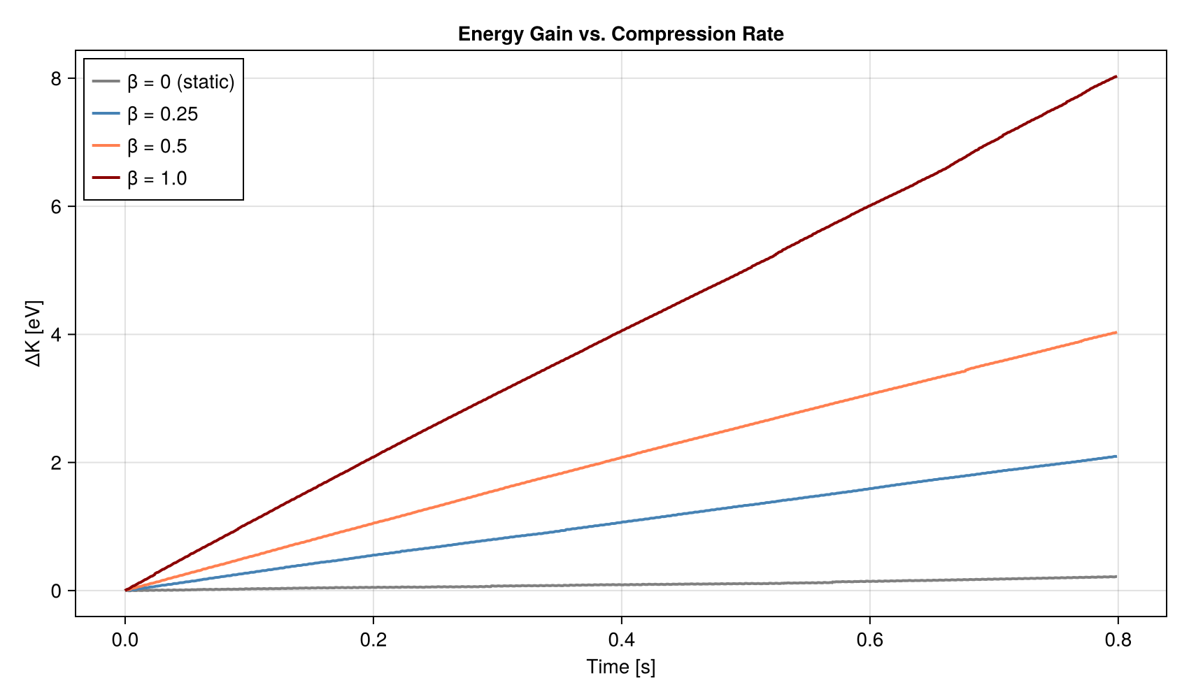

The static case (β = 0) isolates Fermi, Grad-B, and $E_{\parallel }$ with mirror-confined trajectories. As β increases, betatron joins as a visible additive channel, with all mechanisms scaling proportionally.