Curvature and Grad-B Drifts

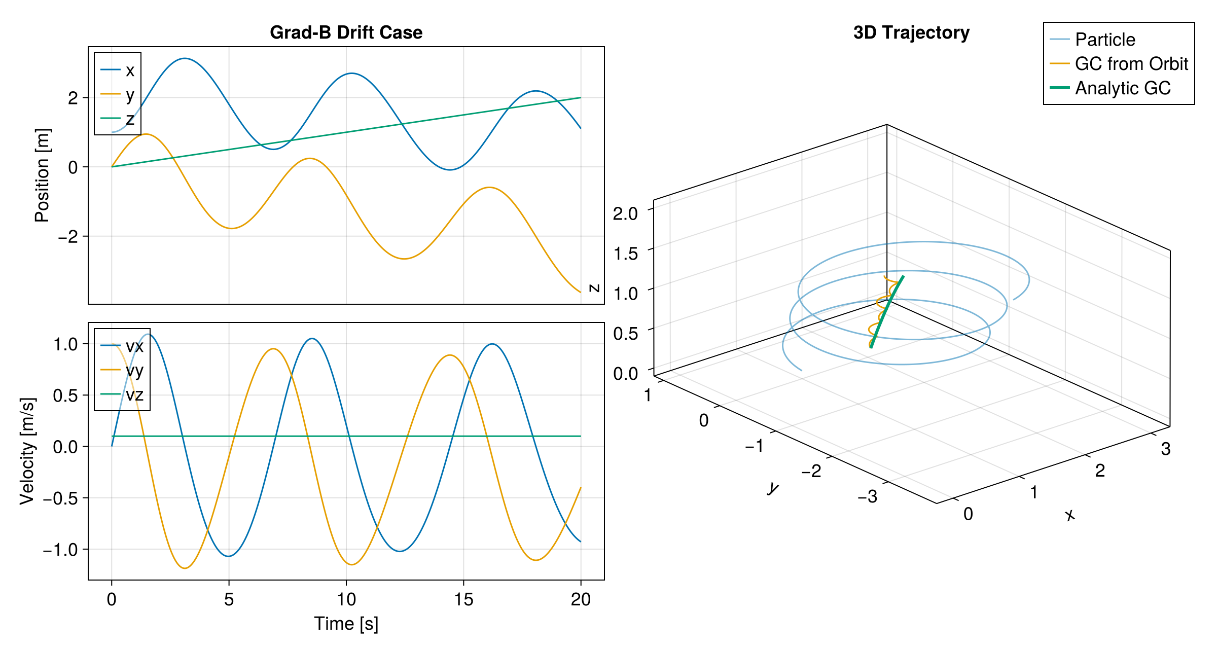
This example demonstrates a single proton motion under two different non-uniform magnetic fields — one with field-line curvature, one with a perpendicular magnitude gradient. Both are more complex than the simpler ExB Drift. For each field we trace the full orbit and compare the guiding center (GC) obtained from the orbit with the analytic GC.

• Curvature drift comes from a curved field line, κ = (b·∇)b; the GC is traced with trace_gc_drifts!.

• Grad-B drift comes from ∇B ⊥ B; the analytic GC is traced with the same trace_gc_drifts! and also carries the ExB drift.

In both cases the orbit-derived GC (the instantaneous guiding center obtained by applying the GC transformation to each point of the full particle orbit) and the analytic GC (the trajectory integrated from the first-order drift formulas) follow different trajectories. They agree only to first order: the analytic drifts in trace_gc_drifts! omit the higher-order (FLR) terms, so the two trajectories slowly diverge as the gyration phase accumulates.

The combined effect of the two drifts for one particle is validated in Magnetic Drift and Energy Partition, and their relation at the particle and fluid level is discussed in Relation between the Magnetic Drifts.

More theoretical details can be found in Curvature/Grad-B Drift, and Fundamentals of Plasma Physics by Paul Bellan.

using TestParticle, OrdinaryDiffEq, StaticArrays
using LinearAlgebra: ×, ⋅, normalize, norm
using CairoMakie

Plotting function

For a traced orbit sol and its analytic GC sol_gc, draw the time series on the left and the 3D trajectory (particle, GC from orbit, analytic GC) on the right, into a dedicated figure.

function plot_drift_case(sol, sol_gc, title)
    fig = Figure(size = (1200, 640), fontsize = 18)

    gl_left = fig[1, 1] = GridLayout()
    ax_pos = Axis(gl_left[1, 1], ylabel = "Position [m]", title = title)
    lines!(ax_pos, sol, idxs = (0, 1), label = "x")
    lines!(ax_pos, sol, idxs = (0, 2), label = "y")
    lines!(ax_pos, sol, idxs = (0, 3), label = "z")
    axislegend(
        ax_pos, position = :lt, framevisible = true,
        backgroundcolor = (:white, 0.5)
    )
    hidexdecorations!(ax_pos, grid = false)

    ax_vel = Axis(gl_left[2, 1], xlabel = "Time [s]", ylabel = "Velocity [m/s]")
    lines!(ax_vel, sol, idxs = (0, 4), label = "vx")
    lines!(ax_vel, sol, idxs = (0, 5), label = "vy")
    lines!(ax_vel, sol, idxs = (0, 6), label = "vz")
    axislegend(
        ax_vel, position = :lt, framevisible = true,
        backgroundcolor = (:white, 0.5)
    )

    linkxaxes!(ax_pos, ax_vel)

    ax_3d = Axis3(
        fig[1, 2]; title = "3D Trajectory", xlabel = "x",
        ylabel = "y", zlabel = "z", aspect = :data
    )

    gc = get_gc_func(sol_gc.prob.p)
    gc_plot(x, y, z, vx, vy, vz) = (gc(SA[x, y, z, vx, vy, vz])...,)

    lines!(
        ax_3d, sol; idxs = (1, 2, 3), color = Makie.wong_colors()[1],
        alpha = 0.5, label = "Particle"
    )
    lines!(
        ax_3d, sol; idxs = (gc_plot, 1, 2, 3, 4, 5, 6),
        color = Makie.wong_colors()[2], label = "GC from Orbit"
    )
    lines!(
        ax_3d, sol_gc; idxs = (1, 2, 3), color = Makie.wong_colors()[3],
        linewidth = 3, label = "Analytic GC"
    )
    axislegend(ax_3d, framevisible = true, backgroundcolor = (:white, 0.5))

    return fig
end;

Curvature B field

A 2D azimuthal field circling the z-axis with radius r: B = B₀ (x₂, -x₁, 0) / r². It has a curved field line (R_c = r) and a radial magnitude gradient, so both curvature and grad-B drifts contribute. We trace a proton with a small v_z so the resulting drift is visible.

curved_B(x) = SA[x[2] / norm(x[1:2])^2, -x[1] / norm(x[1:2])^2, 0.0] * 1.0e-8
zero_E(x) = SA[0.0, 0.0, 0.0]

stateinit_curv = let x0 = [1.0, 0.0, 0.0], v0 = [0.0, 1.0, 0.1]
    [x0..., v0...]
end
tspan_curv = (0, 40)
param_curv = prepare(zero_E, curved_B, species = Proton)
prob_curv = ODEProblem(trace!, stateinit_curv, tspan_curv, param_curv)
sol_curv = solve(prob_curv, Vern9())
gc_curv = param_curv |> get_gc_func
gc_x0_curv = gc_curv(stateinit_curv) |> Vector
prob_gc_curv = ODEProblem(
    trace_gc_drifts!, gc_x0_curv, tspan_curv,
    (param_curv..., sol_curv)
)
sol_gc_curv = solve(prob_gc_curv, Vern7(); save_idxs = [1, 2, 3]);

The orbit-derived and analytic GCs follow different trajectories, because the analytic GC uses only the first-order drift formula and misses the higher-order (FLR) terms that the orbit-derived GC carries.

fig_curv = plot_drift_case(sol_curv, sol_gc_curv, "Curvature Drift Case")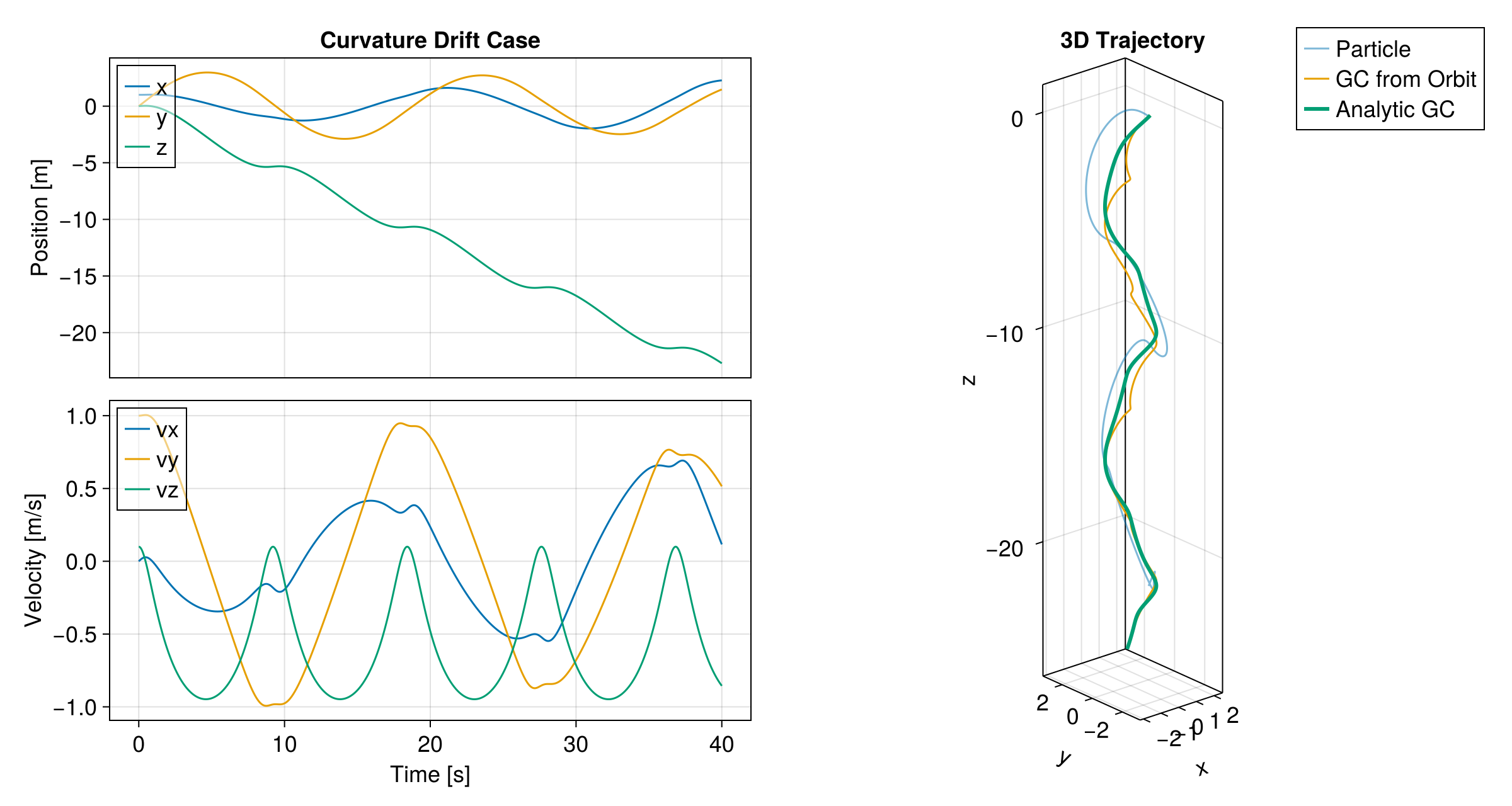

Grad-B field

A straight field B = B₀(1 + g·x₂) ẑ with a perpendicular gradient, plus a small uniform E so the analytic GC also carries the ExB drift. The GC is traced with the library trace_gc_drifts! — the same routine used for the curvature case above — which includes the grad-B, curvature, and ExB drifts (the curvature term vanishes for this straight field).

grad_B(x) = SA[0, 0, 1.0e-8 + 1.0e-9 * x[2]]
uniform_E(x) = SA[1.0e-9, 0, 0]

stateinit_grad = let x0 = [1.0, 0, 0], v0 = [0.0, 1.0, 0.1]
    [x0..., v0...]
end
tspan_grad = (0, 20)
param_grad = prepare(uniform_E, grad_B, species = Proton)
prob_grad = ODEProblem(trace!, stateinit_grad, tspan_grad, param_grad)
sol_grad = solve(prob_grad, Vern9())
gc_grad = param_grad |> get_gc_func
gc_x0_grad = gc_grad(stateinit_grad) |> Vector
prob_gc_grad = ODEProblem(
    trace_gc_drifts!, gc_x0_grad, tspan_grad,
    (param_grad..., sol_grad)
)
sol_gc_grad = solve(prob_gc_grad, Vern7(); save_idxs = [1, 2, 3]);

As in the curvature case, the orbit-derived and analytic GCs diverge, for the same reason: the analytic GC is the first-order drift trajectory, while the orbit-derived GC also carries the higher-order terms beyond the textbook formula.

fig_grad = plot_drift_case(sol_grad, sol_gc_grad, "Grad-B Drift Case")