Gravitational Chaos and Fractal Basins

Three equal masses on a circular equilateral orbit form an exact, time-dependent solution of the Newtonian three-body problem. The configuration repeats every orbit, so the gravitational field seen by a test particle is periodic but never stationary, and the motion in it is chaotic: test particles launched from arbitrarily close points end up on opposite sides of the system.

We release massless particles from a regular grid of initial positions, integrate them in the prescribed time-dependent gravity with TestParticle.jl, and record which primary each particle ends up closest to. The resulting map in initial-condition space has fractal basin boundaries, and pairs of neighbouring trajectories separate exponentially.

Everything below is dimensionless, with G, the primary mass and the orbit radius all set to unity.

using TestParticle
using OrdinaryDiffEq
using StaticArrays
using LinearAlgebra
using CairoMakie

const wc = Makie.wong_colors()

const G = 1.0
const primary_mass = 1.0
const orbit_radius = 1.0
const softening = 0.05;

The circular three-body solution

Put the three primaries on a circle of radius $R$ = orbit_radius, 120° apart and with a common orbital phase. The distance between any two of them is $d=\sqrt{3}R$, and each of the two accelerations acting on a given primary makes an angle of 30° with the inward radial direction. The transverse parts therefore cancel exactly and the radial parts add, so the net acceleration is

$$a=2\frac{Gm}{d^2+{\epsilon }^2}\cos {30}^{\circ }=\frac{\sqrt{3}GmR}{(3R^2+{\epsilon }^2{)}^{3/2}},$$

where softening $\epsilon$ regularises the $1/r^2$ singularity. Equating this to the centripetal acceleration ${\omega }^{2}R$ fixes the angular frequency of the orbit,

$$\omega =\sqrt{\frac{3Gm}{(3R^2+{\epsilon }^2{)}^{3/2}}},$$

which is the value used below. The primaries are prescribed on the circle rather than integrated, so this $\omega$ is what makes their motion an exact solution of the softened three-body problem. The table checks that: the net gravitational acceleration on a primary matches the required centripetal acceleration to machine precision.

const angular_frequency = sqrt(
    3G * primary_mass / (3orbit_radius^2 + softening^2)^(3 / 2)
)
const orbital_period = 2π / angular_frequency
const n_orbits = 3
const final_time = n_orbits * orbital_period

function primary_position(i, t)
    phase = angular_frequency * t + 2π * (i - 1) / 3
    return SA[
        orbit_radius * cos(phase),
        orbit_radius * sin(phase),
        0.0,
    ]
end

function gravity(x, t)
    r = SA[x[1], x[2], x[3]]
    acceleration = zero(r)
    for i in 1:3
        displacement = r - primary_position(i, t)
        distance_squared = displacement ⋅ displacement + softening^2
        acceleration -= G * primary_mass * displacement / distance_squared^(3 / 2)
    end
    return acceleration
end

const orbit_mismatch = let r = primary_position(1, 0.0)
    norm(gravity(r, 0.0) + angular_frequency^2 * r) / (angular_frequency^2 * orbit_radius)
end

$omega$	Orbital period $T$	Force mismatch
0.7594	8.2743	2.9e-16

Gravity as an external force

prepare returns (q2m, m, E, B, F), and the equation of motion it defines is

$$\frac{\mathrm{d}\mathbf{v}}{\mathrm{d}t}=\frac{q}{m}(\mathbf{E}+\mathbf{v}\times \mathbf{B})+\frac{\mathbf{F}}{m}.$$

Gravity belongs in the external-force slot F, not in E: E is a force per unit charge and carries no mass. Setting q = 0 switches the Lorentz term off altogether, and m = 1 makes F / m exactly the acceleration returned by gravity. Leaving m at its default proton value would instead divide the acceleration by $m_p$ and blow the integration up.

With no magnetic field there is nothing for a Boris pusher to do, so an ordinary ODE solver is used from here on.

param = prepare(ZeroField(), ZeroField(), gravity; q = 0.0, m = 1.0)

(0.0, 1.0, ZeroField(), ZeroField(), Field with interpolation support
Time-dependent: true
)

Fractal outcome map

Every grid point is the initial position of a particle released from rest in the $z=0$ plane, integrated for n_orbits orbits. Its colour is the index of the primary it is closest to at the end. Since $T$ is a whole number of orbits, the primaries are back at their starting positions at $t=3T$, which makes the three basins directly comparable.

The integration below uses Vern9 rather than the usual Tsit5. At the tight tolerance needed for this problem the higher-order method takes fewer steps, and the two agree grid point for grid point, so the speed-up is free.

const tspan = (0.0, final_time)
const map_limit = 2.0

# `outcome_map(resolution, tspan, param)` traces a `resolution` × `resolution` grid of
# particles released from rest and returns the grid vectors together with the index of
# the primary that each particle ends up closest to.
function outcome_map(resolution, tspan, param)
    xgrid = range(-map_limit, map_limit; length = resolution)
    ygrid = range(-map_limit, map_limit; length = resolution)
    initial_states = [
        SA[x, y, 0.0, 0.0, 0.0, 0.0]
            for y in ygrid for x in xgrid
    ]
    prob_func = (prob, ctx) -> remake(prob; u0 = initial_states[ctx.sim_id])
    prob = TraceProblem(first(initial_states), tspan, param; prob_func)
    endpoints = solve(
        prob, Vern9(), EnsembleThreads(); trajectories = length(initial_states),
        abstol = 1.0e-10, reltol = 1.0e-10, save_everystep = false,
        save_start = false, save_end = true
    )
    outcomes = Matrix{Int}(undef, resolution, resolution)
    for (index, u) in enumerate(endpoints.u)
        endpoint = SA[u[1], u[2], u[3]]
        distances = [
            norm(endpoint - primary_position(i, tspan[2]))
                for i in 1:3
        ]
        outcomes[index] = argmin(distances)
    end
    return xgrid, ygrid, outcomes
end

# The grid is chosen so that its cell size matches `softening`, the length that
# regularises the primary singularities and therefore sets the smallest scale this model
# can resolve at all. Refining beyond that buys picture quality, not physics, so this is
# also a sensible place to stop for runtime.
const resolution = 80
const xgrid, ygrid, outcomes = outcome_map(resolution, tspan, param)

const orbit_times = range(0, orbital_period; length = 400)
const primary_orbits = [[primary_position(i, t) for t in orbit_times] for i in 1:3]

const zoom_limits = (0.2, 1.4, 0.2, 1.4)

fig = Figure(size = (1250, 540))
ax_map = Axis(
    fig[1, 1];
    title = "Nearest primary after $n_orbits orbits",
    xlabel = "x0", ylabel = "y0", aspect = DataAspect()
)
ax_zoom = Axis(
    fig[1, 2];
    title = "Zoom: no scale is smooth",
    xlabel = "x0", ylabel = "y0", aspect = DataAspect()
)
basins = heatmap!(
    ax_map, xgrid, ygrid, outcomes;
    colormap = wc[[1, 2, 3]], colorrange = (1, 3), interpolate = false
)
heatmap!(
    ax_zoom, xgrid, ygrid, outcomes;
    colormap = wc[[1, 2, 3]], colorrange = (1, 3), interpolate = false
)
Legend(
    fig[1, 3],
    [
        MarkerElement(color = wc[i], marker = :rect, markersize = 14)
            for i in 1:3
    ],
    ["Primary 1", "Primary 2", "Primary 3"], "Nearest primary"
)
for ax in (ax_map, ax_zoom)
    for (i, orbit) in enumerate(primary_orbits)
        lines!(
            ax, getindex.(orbit, 1), getindex.(orbit, 2);
            color = :black, linewidth = 1.5, linestyle = :dash
        )
        final_position = primary_position(i, final_time)
        scatter!(ax, [final_position[1]], [final_position[2]]; color = :black, markersize = 8)
    end
end
ax_zoom.limits = zoom_limits
lines!(
    ax_map, [zoom_limits[1], zoom_limits[2], zoom_limits[2], zoom_limits[1], zoom_limits[1]],
    [zoom_limits[3], zoom_limits[3], zoom_limits[4], zoom_limits[4], zoom_limits[3]];
    color = :black, linewidth = 2, linestyle = :dot
)

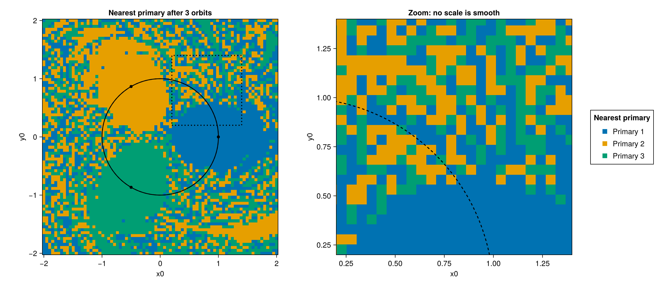
Each primary owns one coherent lobe wrapped in a long filamentary tail, and the three basins are separated by a boundary that interleaves at every scale. Refining the grid does not settle this. If the boundary were a smooth curve, then counting the cell edges across which the label changes and multiplying by the cell size would return a resolution-independent length. Here that product grows with the resolution instead, which is the defining property of a fractal set.

# `boundary_length(outcomes)` is the number of cell edges across which the label
# changes, i.e. the boundary length of the map measured in cells.
function boundary_length(outcomes)
    nx, ny = size(outcomes)
    vertical = sum(
        outcomes[i, j] != outcomes[i + 1, j] for i in 1:(nx - 1), j in 1:ny
    )
    horizontal = sum(
        outcomes[i, j] != outcomes[i, j + 1] for i in 1:nx, j in 1:(ny - 1)
    )
    return vertical + horizontal
end

# Taking every other row and column of the fine map is itself a coarser sample of the
# same initial-condition plane, so the coarse resolution costs nothing to produce.
const resolutions = (resolution ÷ 2, resolution)
const sampled_maps = (outcomes[1:2:end, 1:2:end], outcomes)
const map_statistics = map(zip(resolutions, sampled_maps)) do (res, nres)
    len = boundary_length(nres)
    fractions = [count(==(i), nres) / length(nres) for i in 1:3]
    return (res, len, len * 2 * map_limit / res, fractions)
end

    )

Grid	Boundary length [cells]	Estimated length	Basin 1	Basin 2	Basin 3
40 × 40	1434	143	31.1%	34.7%	34.2%
80 × 80	5358	268	31.6%	34.6%	33.8%

The estimated boundary length grows by roughly a factor of two every time the grid is refined by a factor of two, instead of converging to a finite number. That divergence is what makes the boundary a fractal. The basin areas, on the other hand, are perfectly ordinary: each sits within about two percent of the $1/3$ that the three-fold symmetry demands, and each moves by less than a percent under the refinement. The symmetry fixes the coarse measure of a basin while saying nothing at all about the boundary between them, which is why the areas converge and the boundary length cannot.

Sensitivity to initial conditions

The map above is a finite-time statement, but the motion underneath it is genuinely chaotic. Two particles released d0 apart in $x$ separate exponentially, at a rate set by the flow and not by d0. The particle used below starts from rest inside the filamentary region, where neighbouring cells of the map land in different basins.

const nearby_x0 = SA[0.3, 1.3, 0.0]
const nearby_v0 = SA[0.0, 0.0, 0.0]
const initial_offsets = (1.0e-4, 1.0e-6, 1.0e-8)

# `separation_curve(x0, v0, d0, tspan, param)` traces the pair `(x0, v0)` and
# `(x0 + d0 e_x, v0)` on a common time grid and returns that grid together with the
# position separation at every sample.
function separation_curve(
        x0, v0, d0, tspan, param; nt = 2000, abstol = 1.0e-10, reltol = 1.0e-10
    )
    sample_times = range(tspan[1], tspan[2]; length = nt)
    reference = solve(
        TraceProblem(SA[x0..., v0...], tspan, param), Vern9();
        saveat = sample_times, abstol, reltol
    )
    shifted = solve(
        TraceProblem(SA[x0[1] + d0, x0[2], x0[3], v0...], tspan, param), Vern9();
        saveat = sample_times, abstol, reltol
    )
    distance = [norm(u[1:3] .- w[1:3]) for (u, w) in zip(reference.u, shifted.u)]
    return reference.t, distance, reference, shifted
end

# `growth_rate(d0, distance, final_time)` is the mean exponential amplification rate
# `ln(Δ / d0) / t`, the finite-time estimate of the largest Lyapunov exponent over the
# whole window.
function growth_rate(d0, distance, final_time)
    return log(last(distance) / d0) / final_time
end

const separation_curves = map(initial_offsets) do d0
    times, distance, reference, shifted = separation_curve(
        nearby_x0, nearby_v0, d0, tspan, param
    )
    return (d0, times, distance, reference, shifted)
end

_, _, _, reference, shifted = separation_curves[2]

fig = Figure(size = (1250, 500))
ax_traj = Axis(
    fig[1, 1];
    title = "Two particles released 1e-6 apart",
    xlabel = "x", ylabel = "y", aspect = DataAspect()
)
ax_sep = Axis(
    fig[1, 2];
    title = "Exponential separation",
    xlabel = "t / T", ylabel = "pair separation", yscale = log10
)
for orbit in primary_orbits
    lines!(
        ax_traj, getindex.(orbit, 1), getindex.(orbit, 2);
        color = :gray, linewidth = 1.5, linestyle = :dash
    )
end
for (label, sol, color) in (("Reference", reference, wc[1]), ("Perturbed", shifted, wc[2]))
    lines!(ax_traj, sol[1, :], sol[2, :]; linewidth = 2, color, label)
end
scatter!(ax_traj, [nearby_x0[1]], [nearby_x0[2]]; color = :black, markersize = 8)
axislegend(ax_traj; position = :rt, framevisible = false)
ax_traj.limits = (-1.5, 1.5, -1.5, 1.5)
for (i, (d0, times, distance, _, _)) in enumerate(separation_curves)
    lines!(
        ax_sep, times ./ orbital_period, distance;
        linewidth = 2, color = wc[i], label = @sprintf("offset = %.1e", d0)
    )
end
axislegend(ax_sep; position = :lt, framevisible = false)


const separation_rates = map(separation_curves) do (d0, _, distance, _, _)
    (d0, last(distance), last(distance) / d0, growth_rate(d0, distance, final_time))
end

Offset $delta_0$	Separation at 3 $T$	Gain	E-foldings per orbit
1.0e-04	1.29e+00	1.3e+04	3.2
1.0e-06	6.84e-01	6.8e+05	4.5
1.0e-08	4.46e-03	4.5e+05	4.3

Whatever the initial offset, over three orbits the pair gains four to six orders of magnitude in separation, which is roughly three to five e-foldings per orbit. The amplification factor is therefore the same for offsets that differ by four orders of magnitude: it is a property of the flow, not of the perturbation, and it is a finite-time estimate of the largest Lyapunov exponent of the underlying time-periodic three-body problem. The three curves are not straight over the whole window because the growth is only intermittently exponential and saturates once the pair is a distance apart comparable to the system size.

None of this is an integrator artifact, but it does require the tolerance to be small compared with the separation being resolved. Re-running the ${\delta }_0={10}^{-6}$ pair with progressively tighter tolerances moves the final separation by about a percent, and once the tolerance reaches ${10}^{-10}$ by less than one part in ${10}^4$.

const tolerances = (1.0e-8, 1.0e-10, 1.0e-12)
const tolerance_summary = map(tolerances) do tol
    _, distance, _, _ = separation_curve(
        nearby_x0, nearby_v0, 1.0e-6, tspan, param; abstol = tol, reltol = tol
    )
    return (tol, last(distance))
end

abstol = reltol	Separation at 3 $T$
1e-08	0.676848
1e-10	0.684032
1e-12	0.684147

The pair released ${10}^{-8}$ apart needs a tolerance well below that offset, and the ${\delta }_0={10}^{-6}$ pair needs it to be converged, which is what the table checks. At the default tolerances the same two trajectories would simply follow numerical noise.

This is a softened, dimensionless model of a finite-time outcome map. The primaries are prescribed rather than integrated, softening sets the innermost scale of the filamentary structure, and neither the map nor the Lyapunov rate should be read as an infinite-time, infinite-resolution limit.