Relation between the Magnetic Drifts

A charged particle in a non-uniform magnetic field has two distinct drift contributions that are usually discussed separately:

• grad-B drift \propto v_\perp^2, driven by the field magnitude gradient ∇B;

• curvature drift \propto v_\parallel^2, driven by the field-line curvature κ = (b·∇)b.

Their vector sum is the total magnetic drift. The standalone demos Curvature and Grad-B Drifts and Magnetic Drift and Energy Partition show each drift in detail (trajectories, guiding centre, pitch-angle partition). This demo compares the drifts side by side and shows their relation from three angles:

• Single particle: the two drifts are really one drift split by the kinetic-energy partition v_\perp^2 vs v_\parallel^2 — they add vectorially to the total.

• Fluid average: averaged over an ensemble the total depends only on p_\parallel + p_\perp, so the grad-B and curvature pieces are not separately resolvable.

• Magnetization current: in a fluid the grad-B drift is exactly the diamagnetic current, while the curvature drift survives as a residual. This is the resolution of issue #61.

Shared field

Both parts use the coupled 2D azimuthal field B = B₀(x₂,-x₁,0)/r², where grad-B and curvature are linked through B·R_c = B₀, so the relation is clean. We add a pure grad-B straight field for the fluid-level current identity.

using TestParticle, OrdinaryDiffEq, StaticArrays
using LinearAlgebra: norm, ×, ⋅, normalize
using Statistics: mean
using Random: MersenneTwister
using ForwardDiff: jacobian
using CairoMakie

const Bmag0 = 1.0e-7
curve_B(x) = SA[x[2] / norm(x[1:2])^2, -x[1] / norm(x[1:2])^2, 0.0] * Bmag0
zero_E(x) = SA[0.0, 0.0, 0.0]
x0 = SA[1.0, 0.0, 0.0]
b0 = normalize(curve_B(x0))      # b = (0, -1, 0) at x0
eperp = SA[0.0, 0.0, 1.0]        # perpendicular to b at x0
q, m = Proton.q, Proton.m
coef = m / (q * Bmag0)           # |v_drift| = coef·(v_∥² + v_⊥²/2)

0.10439684914853153

Single-particle drift: one drift split by energy

For a given particle the guiding-centre magnetic drift is the vector sum of a grad-B part (\propto v_\perp^2) and a curvature part (\propto v_\parallel^2). In this field both b×∇B and b×κ point along -ẑ, so the two parts are collinear and we can compare them directly. We evaluate them from the field using the same quantities (∇B, κ) as the package's trace_gc_drifts!.

function magnetic_drift_parts(x, v, q, m)
    B = curve_B(x); Bmag = norm(B); b = B / Bmag
    JB = jacobian(curve_B, x)
    ∇B = JB' * b
    κ = (JB * b + b * (-(∇B ⋅ b))) / Bmag
    Ω = (q / m) * Bmag
    vpar = v ⋅ b; vperp = v - vpar * b; wsq = vperp ⋅ vperp
    v_gB = wsq * (b × ∇B) / (2Ω * Bmag)     # grad-B drift, ∝ v_⊥²
    v_curv = vpar^2 * (b × κ) / Ω         # curvature drift, ∝ v_∥²
    return v_gB, v_curv, v_gB + v_curv
end

magnetic_drift_parts (generic function with 1 method)

Three representative particles of the same speed v0: curvature-dominated (v_\parallel = v0), isotropic (v_\parallel = v_\perp), and grad-B-dominated (v_\perp = v0).

const v0 = 1.0
cases_sp = Dict(
    "curvature-dominated (v∥=v0)" => v0 * b0,
    "isotropic (v∥=v⊥)" => (v0 / √2) * b0 + (v0 / √2) * eperp,
    "grad-B-dominated (v⊥=v0)" => v0 * eperp,
)
parts = Dict{String, NTuple{3, Vector{Float64}}}()
for (name, v) in cases_sp
    parts[name] = magnetic_drift_parts(x0, v, q, m)
end
for name in keys(cases_sp)
    vg, vc, vt = parts[name]
    println(
        rpad(name, 28), " v_gB,z = ", round(vg[3], digits = 4),
        "   v_curv,z = ", round(vc[3], digits = 4),
        "   v_total,z = ", round(vt[3], digits = 4)
    )
end

gBp = [-parts[name][1][3] for name in keys(cases_sp)]  # |·| (all along -ẑ)
cvp = [-parts[name][2][3] for name in keys(cases_sp)]
totp = gBp .+ cvp

fig1 = Figure(size = (800, 500), fontsize = 24)
axA = Axis(
    fig1[1, 1]; title = "Drift decomposition for three particles",
    xlabel = "particle", ylabel = "|v_drift,z| [m/s]",
    xticks = (1:3, ["curvature-\ndominated", "isotropic", "grad-B-\ndominated"]),
    xticklabelrotation = π / 6, xticklabelsize = 18
)
barplot!(axA, (1:3) .- 0.2, gBp; width = 0.35, color = :green, label = "grad-B ∝ v⊥²")
barplot!(axA, (1:3) .+ 0.2, cvp; width = 0.35, color = :orange, label = "curvature ∝ v∥²")
scatter!(
    axA, 1:3, totp; color = :black, markersize = 12, marker = :diamond,
    label = "total = sum"
)
axislegend(axA, position = :lt)

Makie.Legend()

The two single-particle drifts are one magnetic drift whose components add up to the total: the curvature-dominated particle carries only the curvature bar, the grad-B- dominated one only the grad-B bar, and the isotropic one carries both; in every case v_total = v_gB + v_curv. Their energy weighting is shown by the pitch-angle fit in Magnetic Drift and Energy Partition.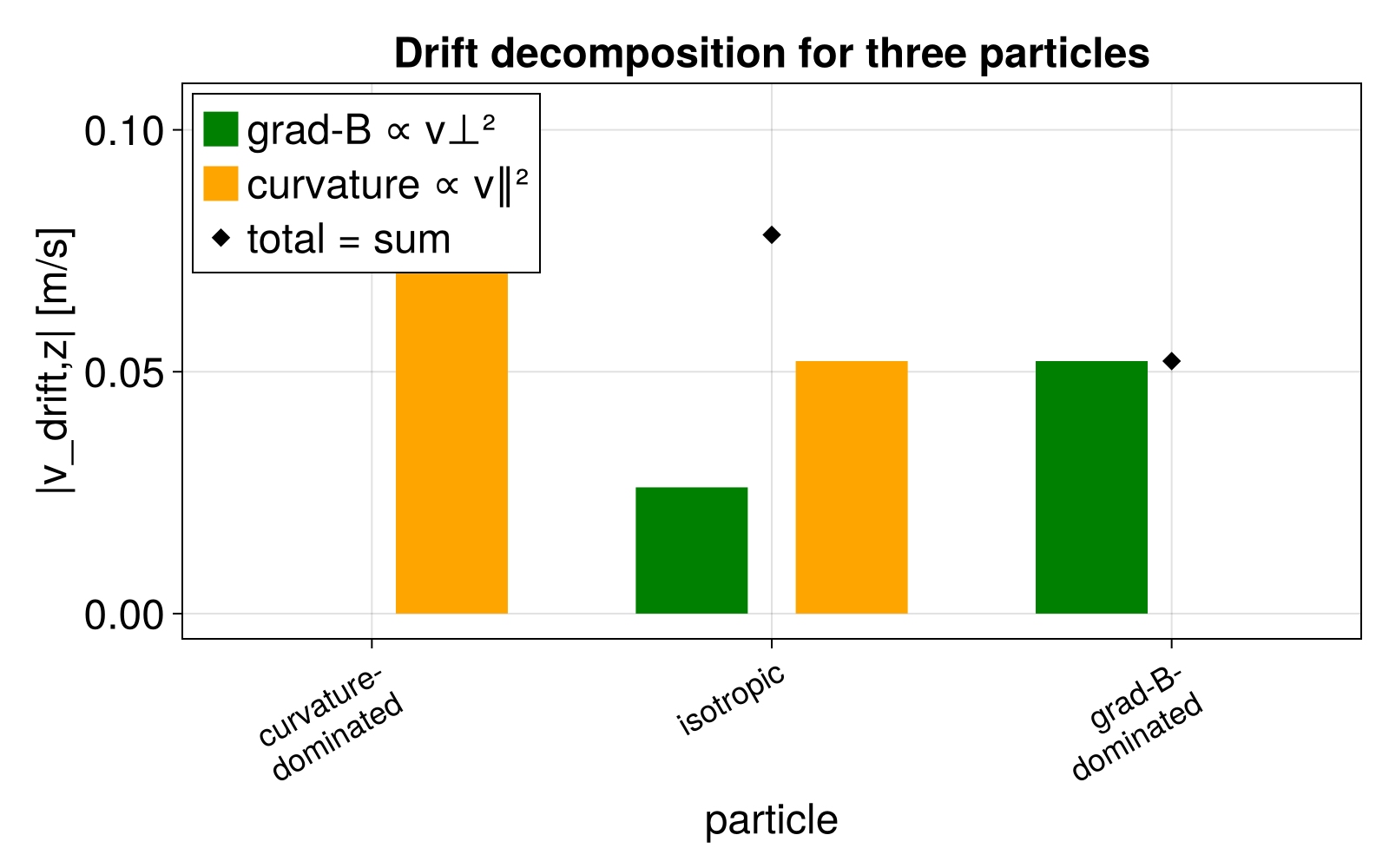

Fluid average: why only one drift appears

Averaged over a (bi-Maxwellian) ensemble the two contributions collapse into one magnetic drift whose magnitude is ⟨v_z⟩ = -coef·(⟨v_∥²⟩ + ⟨v_⊥²⟩/2), so it depends only on p_∥ + p_⊥. Swapping p_∥ and p_⊥ reweights the two pieces but leaves the measured total unchanged, so the fluid moment cannot resolve them separately.

function sample_ensemble(Tpar, Tperp, N; seed = 20240720)
    rng = MersenneTwister(seed)
    vs = Vector{typeof(x0)}(undef, N)
    for i in 1:N
        vpar = randn(rng) * sqrt(Tpar)
        v1 = randn(rng) * sqrt(Tperp)
        v2 = randn(rng) * sqrt(Tperp)
        vs[i] = vpar * b0 + v1 * eperp + v2 * (b0 × eperp)
    end
    return vs
end

sample_ensemble (generic function with 1 method)

Measured guiding-center drift: slope of z_gc(t) over the orbit (averages out the gyration phase).

function ensemble_drift(vs)
    drifts = Float64[]
    param = prepare(zero_E, curve_B, species = Proton)
    gc = get_gc_func(param)
    ts = range(0.0, 30.0; length = 250)
    A = hcat(ones(length(ts)), ts)
    for v in vs
        sol = solve(
            ODEProblem(trace!, [x0..., v...], (0.0, 30.0), param), Vern9();
            abstol = 1.0e-9, reltol = 1.0e-9
        )
        gcz = [gc(sol(t))[3] for t in ts]
        push!(drifts, (A \ gcz)[2])
    end
    return mean(drifts)
end

N = 120
cases = Dict(
    "isotropic (T∥=T⊥=1)" => (1.0, 1.0),
    "bi-Max (T∥=2, T⊥=1)" => (2.0, 1.0),
    "bi-Max (T∥=1, T⊥=2)" => (1.0, 2.0),
)
meas = Dict{String, Float64}()
an = Dict{String, Float64}()
for (name, (Tpar, Tperp)) in cases
    vs = sample_ensemble(Tpar, Tperp, N)
    meas[name] = ensemble_drift(vs)
    an[name] = -coef * (Tpar + Tperp)   # ⟨v_∥²⟩ = Tpar, ⟨v_⊥²⟩ = 2 Tperp
end
for name in keys(cases)
    println(
        rpad(name, 24), " measured = ", round(meas[name], digits = 4),
        "   analytic = ", round(an[name], digits = 4)
    )
end

fig2 = Figure(size = (1600, 500), fontsize = 22)

ax1 = Axis(
    fig2[1, 1]; title = "Ensemble-averaged drift vz",
    xlabel = "case", ylabel = "⟨v_gc,z⟩ [m/s]", xticks = (1:3, collect(keys(cases)))
)
barplot!(ax1, 1:3, [meas[n] for n in keys(cases)]; color = :steelblue, label = "measured")
barplot!(ax1, 1:3, [an[n] for n in keys(cases)]; color = :red, label = "analytic sum of drifts")
axislegend(ax1, position = :lb, ncols = 3)

ax2 = Axis(
    fig2[1, 2]; title = "Pressure-weighted decomposition",
    xlabel = "case", ylabel = "drift contribution [m/s]",
    xticks = (1:3, collect(keys(cases)))
)
curv = [-coef * Tpar for (_, (Tpar, _)) in cases]
grad = [-coef * Tperp for (_, (_, Tperp)) in cases]
barplot!(ax2, (1:3) .- 0.2, curv; width = 0.4, color = :orange, label = "curvature ∝ p∥")
barplot!(ax2, (1:3) .+ 0.2, grad; width = 0.4, color = :green, label = "grad-B ∝ p⊥")
axislegend(ax2, position = :lb, ncols = 3)

ax3 = Axis3(
    fig2[1, 3]; title = "Sample trajectories", xlabel = "x", ylabel = "y",
    zlabel = "z", aspect = :data
)
vs_iso = sample_ensemble(1.0, 1.0, 1; seed = 1)
vs_an = sample_ensemble(2.0, 1.0, 1; seed = 2)
for (lab, v) in [("isotropic", vs_iso[1]), ("bi-Max (T∥>T⊥)", vs_an[1])]
    param = prepare(zero_E, curve_B, species = Proton)
    sol = solve(
        ODEProblem(trace!, [x0..., v...], (0.0, 30.0), param), Vern9();
        abstol = 1.0e-9, reltol = 1.0e-9
    )
    lines!(ax3, sol; idxs = (1, 2, 3), label = lab)
end
axislegend(ax3, framevisible = true, backgroundcolor = (:white, 0.6));

bi-Max (T∥=1, T⊥=2)      measured = -0.3279   analytic = -0.3132
bi-Max (T∥=2, T⊥=1)      measured = -0.3255   analytic = -0.3132
isotropic (T∥=T⊥=1)      measured = -0.2207   analytic = -0.2088

The total fluid-level drift depends on Tpar + Tperp (the pressure), not separately on grad-B or curvature: the two bi-Maxwellian cases have the same measured drift (left), even though their internal curvature/grad-B split is swapped (middle). The averaged magnetic drift is a single quantity at the fluid level.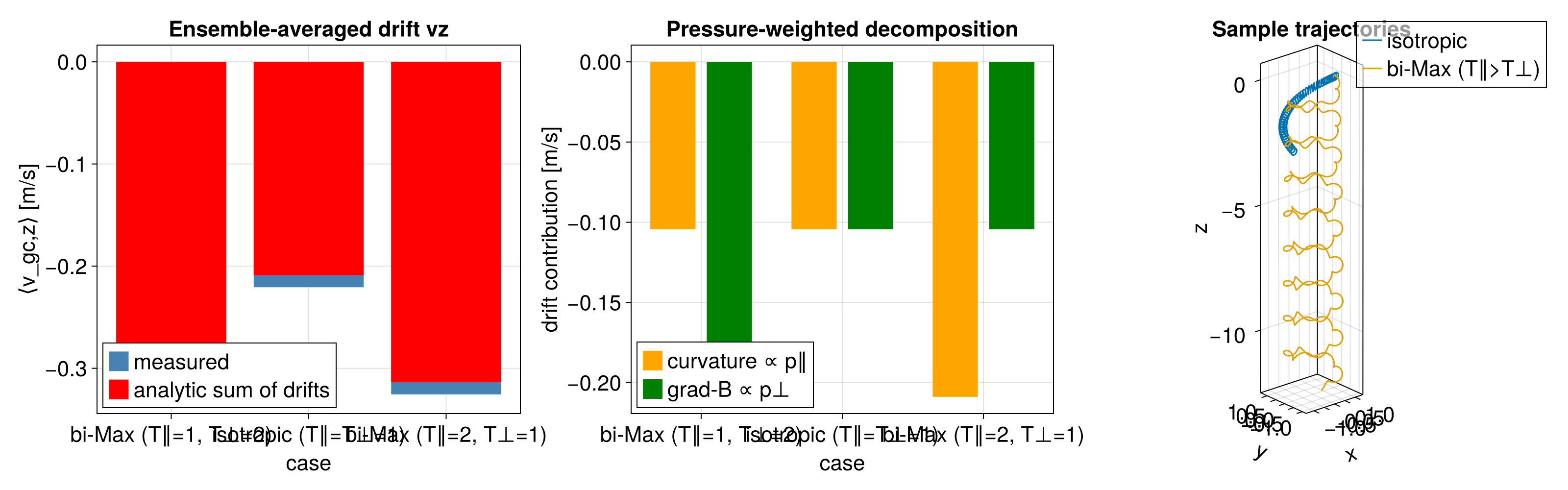

The magnetization current: where the grad-B drift goes

A gyrating particle carries a magnetic moment μ = m v_⊥²/(2B), whose inhomogeneity produces a magnetization current J_mag = ∇×(nμb). For a pure grad-B field the grad-B drift current is exactly the magnetization (diamagnetic) current: J_∇B = J_mag = J_diam. So grad-B is not an independent fluid current — it already is the diamagnetic current. Because μ depends only on v_⊥², J_mag carries the grad-B piece and nothing else; the curvature drift (∝ v_∥²) has no magnetization twin and survives as the residual centrifugal current.

We compute these directly from the field, using the same drift quantities (∇B, κ, b) the package evaluates in trace_gc_drifts!. Units are normalized (m = q = n = 1); the current identities are scale-independent.

function Bprops(x, Bfunc)
    B = Bfunc(x); Bmag = norm(B); b = B / Bmag
    JB = jacobian(Bfunc, x)
    ∇B = JB' * b
    κ = (JB * b + b * (-(∇B ⋅ b))) / Bmag
    return Bmag, b, ∇B, κ
end

# Numerical curl of a vector field at `x0` (central differences).
function curl(F, x0, δ = 1.0e-4)
    fx(off, i, k) = (x = Vector(x0); x[i] += off; F(x)[k])
    C = SA[
        (fx(δ, 2, 3) - fx(-δ, 2, 3) + fx(-δ, 3, 2) - fx(δ, 3, 2)) / (2δ),
        (fx(δ, 3, 1) - fx(-δ, 3, 1) + fx(-δ, 1, 3) - fx(δ, 1, 3)) / (2δ),
        (fx(δ, 1, 2) - fx(-δ, 1, 2) + fx(-δ, 2, 1) - fx(δ, 2, 1)) / (2δ),
    ]
    return C
end

curl (generic function with 2 methods)

Drift currents from the guiding-centre formula (perpendicular, ensemble-averaged). J_∇B = n·m·⟨v_⊥²⟩ (b×∇B) / (2B²) (∝ v_⊥²) J_curv = n·m·⟨v_∥²⟩ (b×κ) / B (∝ v_∥²)

function drift_currents(x, Bfunc; Tpar, Tperp, n = 1.0, m = 1.0)
    (Bmag, b, ∇B, κ) = Bprops(x, Bfunc)
    vperp2 = 2Tperp; vpar2 = Tpar
    Jg = n * m * vperp2 * (b × ∇B) / (2 * Bmag^2)
    Jc = n * m * vpar2 * (b × κ) / Bmag
    return Jg, Jc, Bmag, b
end;

Magnetization current from μ = m⟨v_⊥²⟩/(2B), and the diamagnetic current from the perpendicular pressure p_⊥ = n·m·⟨v_⊥²⟩/2.

function mag_current(x0, Bfunc; Tperp, n = 1.0, m = 1.0)
    vperp2 = 2Tperp
    Mfun(x) = (Bx = Bfunc(x); Bn = norm(Bx); n * (m * vperp2 / (2 * Bn)) * Bx / Bn)
    return curl(Mfun, x0)
end

function diamag_current(x0, Bfunc; Tperp, n = 1.0, m = 1.0)
    p_perp = n * m * (2Tperp) / 2
    F(x) = (Bx = Bfunc(x); Bn = norm(Bx); p_perp * Bx / (Bn * Bn))
    return curl(F, x0)
end

diamag_current (generic function with 1 method)

Pure grad-B straight field (κ = 0)

B = B₀(1 + g·x₂) ẑ. There is no curvature, so only the grad-B drift exists. The ensemble-averaged grad-B drift current must equal the magnetization (and diamagnetic) current.

B0g = 1.0; g = 1.0e-2
gradB_straight(x) = B0g * (1 + g * x[2]) * SA[0.0, 0.0, 1.0]
JgA, _, _, _ = drift_currents(x0, gradB_straight; Tpar = 1.0, Tperp = 1.0)
JmA = mag_current(x0, gradB_straight; Tperp = 1.0)
JdA = diamag_current(x0, gradB_straight; Tperp = 1.0)
println("Pure grad-B straight field (κ = 0):")
println("  |J_∇B|   = ", norm(JgA))
println("  |J_mag|  = ", norm(JmA), "   |J_∇B - J_mag| = ", norm(JgA - JmA))
println("  |J_diam| = ", norm(JdA), "   |J_∇B - J_diam| = ", norm(JgA - JdA))

Pure grad-B straight field (κ = 0):
  |J_∇B|   = 0.01
  |J_mag|  = 0.009999999999732445   |J_∇B - J_mag| = 2.6755507531728284e-13
  |J_diam| = 0.010000000000287557   |J_∇B - J_diam| = 2.8755643699529543e-13

Coupled curved field: isotropic vs anisotropic

Here both drifts exist. The magnetization current depends only on v_⊥², so raising T_∥ (which only feeds the curvature drift) must leave J_mag unchanged while J_curv grows — the curvature part is the un-absorbed residual.

Jg_iso, Jc_iso, _, _ = drift_currents(x0, curve_B; Tpar = 1.0, Tperp = 1.0)
Jm_iso = mag_current(x0, curve_B; Tperp = 1.0)
Jg_an, Jc_an, _, _ = drift_currents(x0, curve_B; Tpar = 4.0, Tperp = 1.0)
Jm_an = mag_current(x0, curve_B; Tperp = 1.0)
println("\nCoupled curved field, isotropic (T∥=T⊥=1):")
println(
    "  |J_∇B| = ", norm(Jg_iso), "   |J_curv| = ", norm(Jc_iso),
    "   |J_mag| = ", norm(Jm_iso)
)
println("Coupled curved field, anisotropic (T∥=4, T⊥=1):")
println(
    "  |J_∇B| = ", norm(Jg_an), "   |J_curv| = ", norm(Jc_an),
    "   |J_mag| = ", norm(Jm_an), "  (unchanged: tracks T⊥ only)"
)

fig3 = Figure(size = (1400, 500), fontsize = 22)

axA = Axis(
    fig3[1, 1]; title = "Pure grad-B field: grad-B drift = diamagnetic current",
    xlabel = "current", ylabel = "magnitude",
    xticks = (1:3, ["J_∇B", "J_mag", "J_diamag"]),
    xgridvisible = false, ygridvisible = false
)
# The three currents coincide (J_∇B = J_mag = J_diamag), so the bars share one height.
barplot!(axA, 1, norm(JgA); width = 0.6, color = :steelblue, label = "J_∇B (drift)")
barplot!(axA, 2, norm(JmA); width = 0.6, color = :green, label = "J_mag (magnetization)")
barplot!(axA, 3, norm(JdA); width = 0.6, color = :orange, label = "J_diamag (pressure)")
axislegend(axA, position = :rt, ncols = 3)

axB = Axis(
    fig3[1, 2]; title = "Curved field: only curvature survives anisotropy",
    xlabel = "case", ylabel = "current magnitude",
    xticks = (1:2, ["isotropic T∥=T⊥=1", "anisotropic T∥=4,T⊥=1"])
)
barplot!(axB, 1 - 0.2, norm(Jg_iso); width = 0.25, color = :steelblue, label = "J_∇B ∝ v⊥²")
barplot!(axB, 1 + 0.0, norm(Jc_iso); width = 0.25, color = :red, label = "J_curv ∝ v∥²")
barplot!(axB, 1 + 0.2, norm(Jm_iso); width = 0.25, color = :green, label = "J_mag ∝ v⊥²")
barplot!(axB, 2 - 0.2, norm(Jg_an); width = 0.25, color = :steelblue)
barplot!(axB, 2 + 0.0, norm(Jc_an); width = 0.25, color = :red)
barplot!(axB, 2 + 0.2, norm(Jm_an); width = 0.25, color = :green)
axislegend(axB, position = :lt, ncols = 3);

Coupled curved field, isotropic (T∥=T⊥=1):
  |J_∇B| = 1.0000000000000002e7   |J_curv| = 1.0e7   |J_mag| = 1.9999999999990687e7
Coupled curved field, anisotropic (T∥=4, T⊥=1):
  |J_∇B| = 1.0000000000000002e7   |J_curv| = 4.0e7   |J_mag| = 1.9999999999990687e7  (unchanged: tracks T⊥ only)

In the pure grad-B field the three currents coincide — the grad-B drift is the diamagnetic current (left). In the curved field, raising T_∥ grows the curvature current J_curv but not the magnetization current J_mag (which only carries the grad-B/v_⊥² piece); the curvature drift is the surviving residual (right). The grad-B drift is absorbed into the diamagnetic current (it is the magnetization current), while the curvature drift survives as the centrifugal current in the single-fluid momentum balance.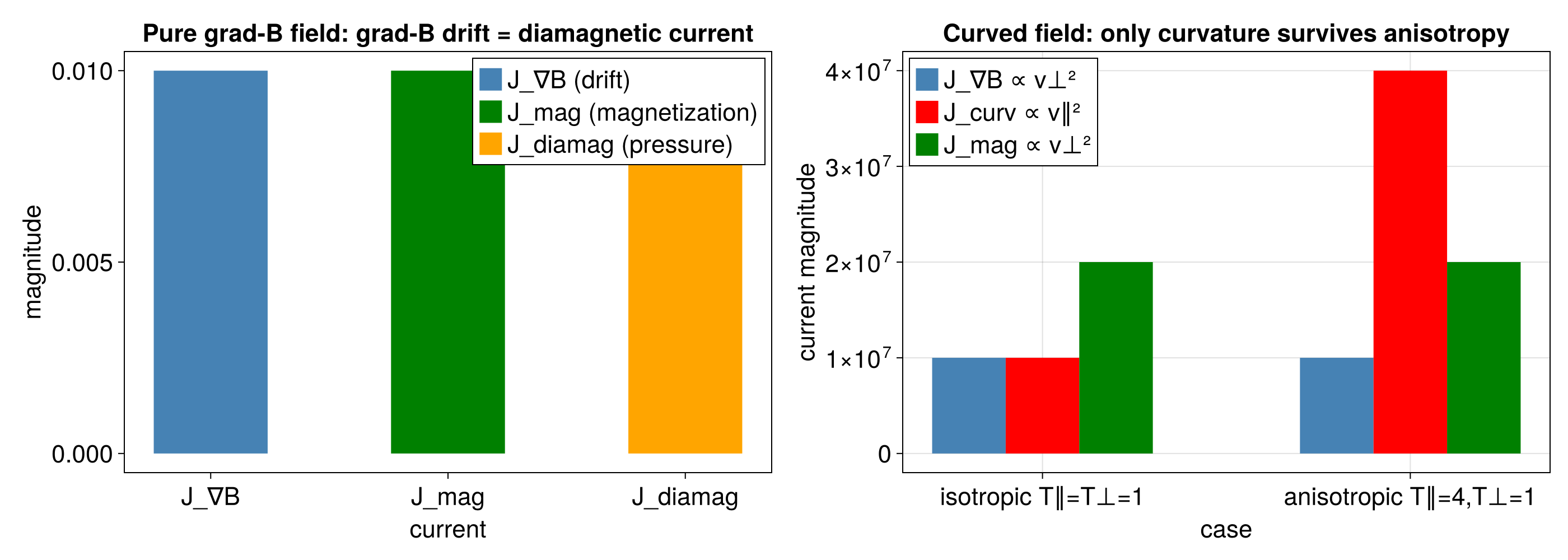

Complete analysis

The single-particle drifts combine into one logical chain. Write the ensemble magnetic-drift current as the sum of its two single-particle pieces (they add vectorially to the total):

$${\mathbf{J}}_m=nm⟨v_{\parallel }^2⟩\frac{\mathbf{b}\times \mathit{\kappa }}{B}+nm\frac{⟨v_{\perp }^2⟩}{2}\frac{\mathbf{b}\times \mathrm{\nabla }B}{B^2}\equiv {\mathbf{J}}_{\mathrm{curv}}+{\mathbf{J}}_{\mathrm{\nabla }B}.$$

The magnetization current shows the second term is not independent: for a gyrating ensemble the grad-B drift current equals the magnetization (diamagnetic) current,

$${\mathbf{J}}_{\mathrm{\nabla }B}=\mathrm{\nabla }\times (n\mu \mathbf{b}),\mu =\frac{m⟨v_{\perp }^2⟩}{2B}⟹{\mathbf{J}}_{\mathrm{\nabla }B}={\mathbf{J}}_{\mathrm{mag}}={\mathbf{J}}_{\mathrm{diam}},$$

while the curvature term ${\mathbf{J}}_{\mathrm{curv}}\propto ⟨v_{\parallel }^2⟩$ has no magnetization twin, because $\mu$ depends only on $v_{\perp }^2$ ( raising $T_{\parallel }$ grows $J_{\mathrm{curv}}$ four-fold but leaves $J_{\mathrm{mag}}$ fixed). Hence

$${\mathbf{J}}_m={\mathbf{J}}_{\mathrm{curv}}+{\mathbf{J}}_{\mathrm{diam}}.$$

The fluid average then shows why the moment cannot see the split: the total drift scales with $⟨v_{\parallel }^2⟩+⟨v_{\perp }^2⟩/2$, i.e. with $p_{\parallel }+p_{\perp }$ (the left panel of the fluid-average figure has identical bars for the two swapped bi-Maxwellian cases, while the middle panel swaps the curvature/grad-B shares). In the single-fluid momentum equation the only place ${\mathbf{J}}_m\times \mathbf{B}$ enters is through the current. The ${\mathbf{J}}_{\mathrm{diam}}\times \mathbf{B}$ part is just the perpendicular pressure-gradient force already carried by the fluid equations; the ${\mathbf{J}}_{\mathrm{curv}}\times \mathbf{B}$ part is the curvature (centrifugal) force. Therefore:

• Curvature drift survives as an explicit centrifugal force in the fluid momentum balance (it is the $\propto v_{\parallel }^2$ residual with no diamagnetic counterpart).

• grad-B drift does not appear separately — it is the diamagnetic current, already accounted for by the pressure term.

This is the complete relation between the magnetic drifts: a single particle has two drifts split by energy, but a fluid carries only one magnetic drift, because grad-B is absorbed into the diamagnetic current while curvature survives.