Magnetic Mirror

This example demonstrates the particle motion trajectory in a magnetic mirror and also illustrates the conservation of magnetic moment. From the third figure on the right, it can be seen that the zero-order quantity of magnetic moment is conserved, but its high-order part is not conserved under this definition of magnetic moment and oscillates rapidly. We can observe from this the oscillation characteristics of magnetic moments at different levels.

This example is based on demo_magneticbottle.jl.

julia

using TestParticle, OrdinaryDiffEq, StaticArrays
import TestParticle as TP
using LinearAlgebra: normalize, norm, ⋅
using CairoMakie

### Obtain field

# Magnetic mirror parameters in SI units
const I = 20.0 # current in the solenoid [A]
const N = 45 # number of windings
const distance = 10.0 # distance between solenoids [m]
const a = 4.0 # radius of each coil [m]

getB(xu) = SVector{3}(TP.getB_mirror(xu[1], xu[2], xu[3], distance, a, I*N))

getE(xu) = SA[0.0, 0.0, 0.0]

# velocity in the direction perpendicular to the magnetic field
function v_perp(t, x, y, z, vx, vy, vz)
   xu = SA[x, y, z, vx, vy, vz]
   vu = @view xu[4:6]
   B = getB(xu)
   b = normalize(B)
   v_pa = (vu ⋅ b) .* b

   (t, norm(vu - v_pa))
end

# magnetic field
absB(t, x, y, z) = (t, sqrt(sum(x -> x^2, getB(SA[x, y, z]))))

# μ, magnetic moment
function mu(t, x, y, z, vx, vy, vz)
   xu = SA[x, y, z, vx, vy, vz]

   (t, v_perp(t, x, y, z, vx, vy, vz)[2]^2 / sqrt(sum(x -> x^2, getB(xu))))
end

Et(xu) = sqrt(xu[4]^2 + xu[5]^2 + xu[6]^2)

### Initialize particles
m = TP.mₑ
q = TP.qₑ
c = TP.c

# initial velocity, [m/s]
v₀ = [2.75, 2.5, 1.3] .* 0.001c  # confined
##v₀ = [0.25, 0.25, 5.9595] .* 0.01c  # escaped
# initial position, [m]
r₀ = [0.8, 0.8, 0.0]  # confined
##r₀ = [1.5, 1.5, 2.4]  # escaped
stateinit = [r₀..., v₀...]

param = prepare(getE, getB; species = Electron)
tspan = (0.0, 1e-4)

prob = ODEProblem(trace!, stateinit, tspan, param)

# Default Tsit5() and many solvers does not work in this case!
# AB4() has better performance in maintaining magnetic moment conservation compared to AB3().
sol_non = solve(prob, AB4(); dt = 3e-9)

### Visualization
f = Figure(size = (900, 600), fontsize = 18)
ax1 = Axis3(f[1:3, 1],
   title = "Magnetic Mirror",
   xlabel = "x [m]",
   ylabel = "y [m]",
   zlabel = "z [m]",
   aspect = :data,
   azimuth = 0.9π,
   elevation = 0.1π
)
ax2 = Axis(f[1, 2], xlabel = "time [s]", ylabel = "B [T]")
ax3 = Axis(f[2, 2], xlabel = "time [s]", ylabel = "v_perp [m/s]")
ax4 = Axis(f[3, 2], xlabel = "time [s]", ylabel = "mu")

lines!(ax1, sol_non, idxs = (1, 2, 3))
lines!(ax2, sol_non, idxs = (absB, 0, 1, 2, 3))
lines!(ax3, sol_non, idxs = (v_perp, 0, 1, 2, 3, 4, 5, 6))
lines!(ax4, sol_non, idxs = (mu, 0, 1, 2, 3, 4, 5, 6))

# Plot coils
θ = range(0, 2π, length = 100)
x = a .* cos.(θ)
y = a .* sin.(θ)
z = fill(distance/2, size(x))
lines!(ax1, x, y, z, color = :red)
z = fill(-distance/2, size(x))
lines!(ax1, x, y, z, color = :red)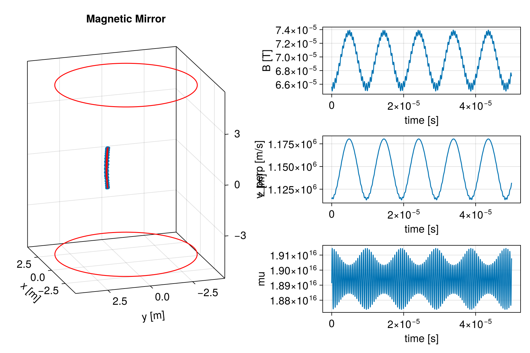

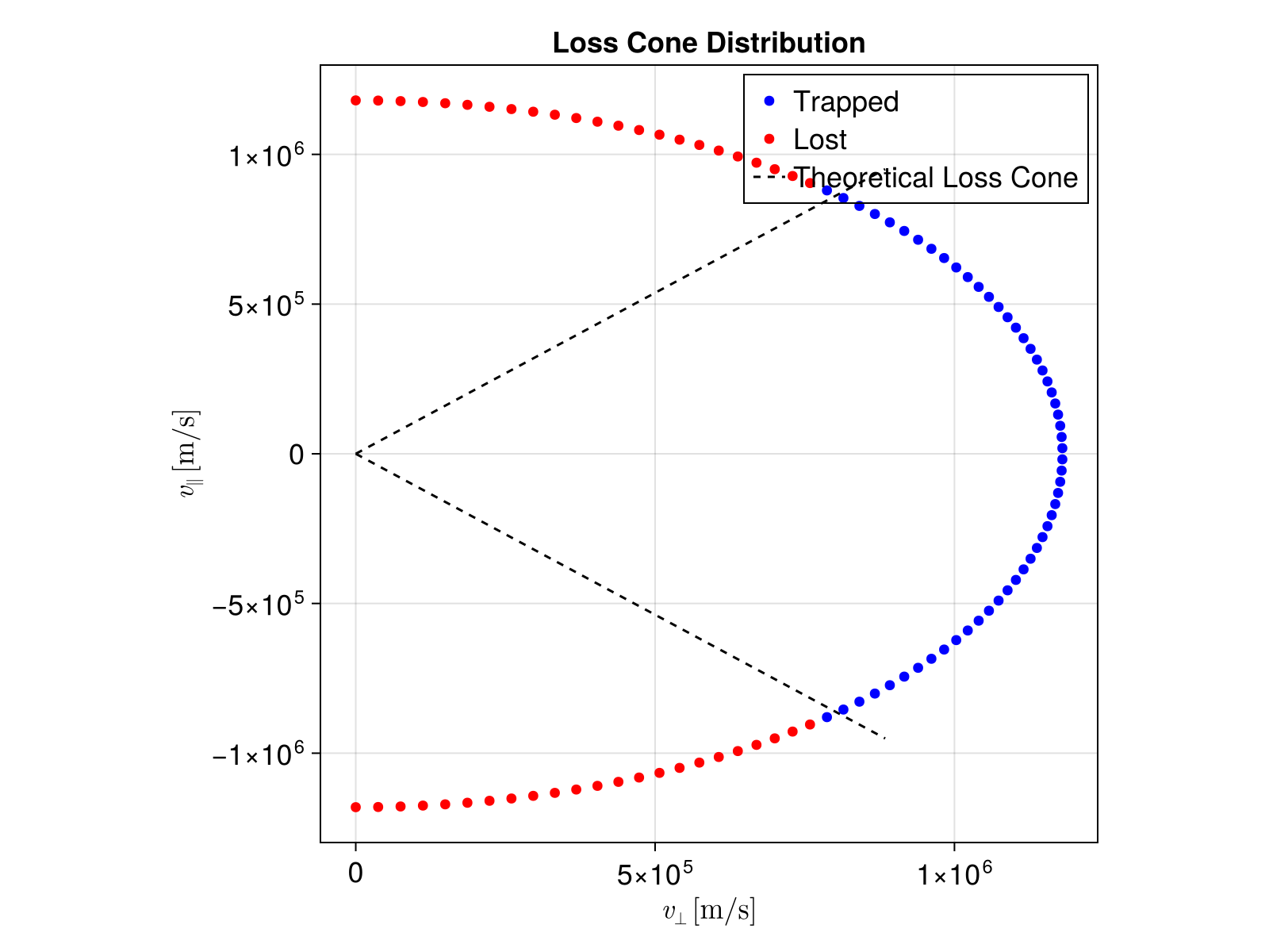
# # The distribution of magnetic field along the z-axis or x-axis
# Bz(z) = hypot(getB(SA[0.0, 0.0, z])...)
# Bx(x) = hypot(getB(SA[x, 0.0, 0.5*distance])...)
# z = collect(-10:0.01:10)
# x = collect(-0.99*a:0.01:0.99*a)
# # Ba = Bz.(z)
# Ba = Bx.(x)
# # lines(z, Ba, color=:red)
# lines(x, Ba, color=:red)

Loss Cone Distribution

We can simulate an ensemble of particles with different pitch angles to visualize the loss cone. The loss cone angle is defined as $α_{l o s s} = \arcsin (\sqrt{B_{m i n} / B_{m a x}})$ . Particles with pitch angle $α < α_{l o s s}$ or $α > π - α_{l o s s}$ will escape the mirror.

julia

# Calculate B_min and B_max
B_min_vec = getB(SA[0.0, 0.0, 0.0])
B_min = norm(B_min_vec)
B_max_vec = getB(SA[0.0, 0.0, distance / 2])
B_max = norm(B_max_vec)
loss_cone_angle = asin(sqrt(B_min / B_max))
println("Loss cone angle: ", rad2deg(loss_cone_angle), "°")

# Define an ensemble of particles
# All particles start at the same radial position r₀ but with different pitch angles.
n_particles = 100
pitch_angles = range(0, π, length = n_particles)
v_mag = norm(v₀)
ensemble_prob = EnsembleProblem(
   prob, prob_func = (prob, i, repeat) -> begin
      α = pitch_angles[i]
      # Velocity components: v_z = v cos(α), v_perp = v sin(α)
      # We put v_perp in x-direction for simplicity
      vz = v_mag * cos(α)
      vx = v_mag * sin(α)
      vy = 0.0
      remake(prob, u0 = [r₀..., vx, vy, vz])
   end)

# Trace particles
# We use a simpler solver for speed and checking escape condition
# We use the `isoutofdomain` check to stop tracing those particles that go out of the mirror structure.
isoutofdomain(u, p, t) = abs(u[3]) > distance/2
callback = DiscreteCallback(isoutofdomain, terminate!)

sim = solve(ensemble_prob, Vern9(), EnsembleThreads(), trajectories = n_particles,
   dt = 3e-9, callback = callback, verbose = false);

Loss cone angle: 42.924519597244355°

Check which particles are trapped A particle is considered trapped if it remains within the mirror (abs(z) < distance/2) Since we stop tracing when they leave, we can check the final position. isoutofdomain rejects the step that goes out, so the final point will be inside. DiscreteCallback accepts the step that goes out, so the final point will be outside. So we need to check if the simulation finished the full time span or was terminated early.

julia

# A robust check here is: if t < tspan[2], it was stopped early (or failed).
is_trapped = map(sim) do sol
   sol.t[end] ≈ tspan[2]
end

# Visualization of Loss Cone
f2 = Figure(size = (800, 600), fontsize = 18)
ax = Axis(f2[1, 1],
   title = "Loss Cone Distribution",
   xlabel = L"v_\perp\,[\mathrm{m/s}]",
   ylabel = L"v_\parallel\,[\mathrm{m/s}]",
   aspect = 1
)

# Extract initial velocities
v_par_init = v_mag .* cos.(pitch_angles)
v_perp_init = v_mag .* sin.(pitch_angles)

# Plot trapped and lost particles
scatter!(
   ax, v_perp_init[is_trapped], v_par_init[is_trapped], label = "Trapped", color = :blue)
scatter!(
   ax, v_perp_init[.!is_trapped], v_par_init[.!is_trapped], label = "Lost", color = :red)

# Draw theoretical loss cone
# v_perp = v_par * tan(alpha) -> v_par = v_perp / tan(alpha)
# Boundary lines: alpha = loss_cone_angle and alpha = pi - loss_cone_angle
max_v = v_mag * 1.1
lines!(ax, [0, max_v * sin(loss_cone_angle)], [0, max_v * cos(loss_cone_angle)],
   color = :black, linestyle = :dash, label = "Theoretical Loss Cone")
lines!(ax, [0, max_v * sin(loss_cone_angle)],
   [0, -max_v * cos(loss_cone_angle)], color = :black, linestyle = :dash)

axislegend(ax, position = :rt, backgroundcolor = :transparent)

Magnetic Mirror ​

Loss Cone Distribution ​

Magnetic Mirror

Loss Cone Distribution