Phase Error Analysis

This example demonstrates how to analyze the phase error of different particle solvers (Boris method and Multistep Boris method) in a simple cyclotron motion. We verify the order of accuracy by plotting the phase error against the time step size.

using TestParticle
using StaticArrays
using LinearAlgebra
using CairoMakie

Test Problem Definition

Define a uniform magnetic field and zero electric field

# Dimensionless units: q=1, m=1, B=1
B_func(x, t) = SA[0.0, 0.0, 1.0]
E_func = TestParticle.ZeroField()

# Parameters
q = 1.0
m = 1.0
Ω = q * 1.0 / m       # Cyclotron frequency
T_period = 2π / Ω     # Cyclotron period

# Initial condition: particle starting at origin with velocity in x-direction
# This results in a circular orbit in the x-y plane.
x0 = [0.0, 0.0, 0.0]
v0 = [1.0, 0.0, 0.0]
u0 = [x0..., v0...]

# Simulation time
# We simulate for multiple periods to allow phase error to accumulate
n_periods = 10
t_end = n_periods * T_period
tspan = (0.0, t_end)

# Prepare the problem parameters
param = prepare(E_func, B_func; species = User, q = q, m = m)
prob = TraceProblem(u0, tspan, param)

# Solvers
# We compare the standard Boris method (n=1) and Multistep Boris method with different substeps.
solvers = [
   ("Boris", 1),
   ("Multistep Boris (n=2)", 2),
   ("Multistep Boris (n=4)", 4)
]

# Time steps to test: decreasing dt
# We choose dt such that we have an integer number of steps per period
steps_per_period = [10, 20, 40, 80, 160, 320]
dts = T_period ./ steps_per_period

# Storage for results
results = Dict(name => Float64[] for (name, _) in solvers)

# Loop over time steps and solvers
for dt in dts
   for (name, n) in solvers
      # Solve the problem
      sol = TestParticle.solve(prob; dt = dt, n = n)[1]

      # Get the final state
      vx = sol.u[end][4]
      vy = sol.u[end][5]
      t_final = sol.t[end]

      # Numerical phase
      # The velocity rotates clockwise in x-y plane for q>0, B_z>0
      # v_x = v_perp * cos(-Ω*t)
      # v_y = v_perp * sin(-Ω*t)
      # phase = -Ω*t
      phi_num = atan(vy, vx)
      phi_ana = -Ω * t_final

      # Calculate phase error
      # We wrap the difference to [-π, π] to handle 2π ambiguity
      diff = phi_num - phi_ana
      phase_error = abs(rem2pi(diff, RoundNearest))

      push!(results[name], phase_error)
   end
end

Visualization

f = Figure(size = (800, 600), fontsize = 18)
ax = Axis(f[1, 1],
   xscale = log10,
   yscale = log10,
   xlabel = "Time step dt",
   ylabel = "Phase Error (rad)",
   title = "Phase Error Convergence ($n_periods periods)",
   xminorticksvisible = true,
   yminorticksvisible = true,
   xgridvisible = true,
   ygridvisible = true
)

for (name, _) in solvers
   scatterlines!(ax, dts, results[name], label = name, linewidth = 2)
end

# Add a reference slope of 2 (2nd order)
# Place it relative to the first data point of Boris
ref_x = dts
ref_y = results["Boris"][1] .* (dts ./ dts[1]) .^ 2
lines!(ax, ref_x, ref_y, label = "2nd Order Ref", linestyle = :dash, color = :black)

axislegend(ax, position = :lt)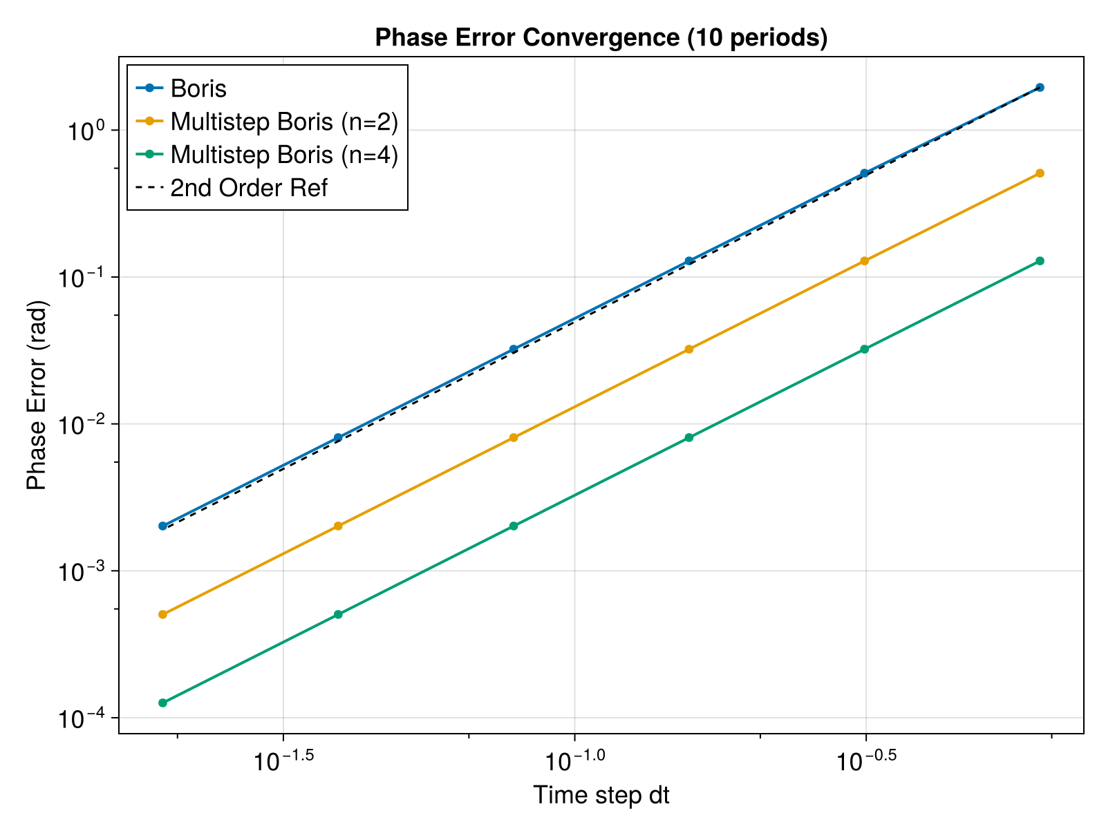

Estimate order of accuracy from slope in log-log plot

println("Estimated Order of Accuracy:")
for (name, _) in solvers
   errors = results[name]
   # Linear regression on log-log data
   X = [ones(length(dts)) log10.(dts)]
   Y = log10.(errors)
   coeffs = X \ Y
   slope = coeffs[2]
   println("$name: $(round(slope, digits=2))")
end

Estimated Order of Accuracy:
Boris: 1.52
Multistep Boris (n=2): 1.25
Multistep Boris (n=4): 1.08