Earth Gravity

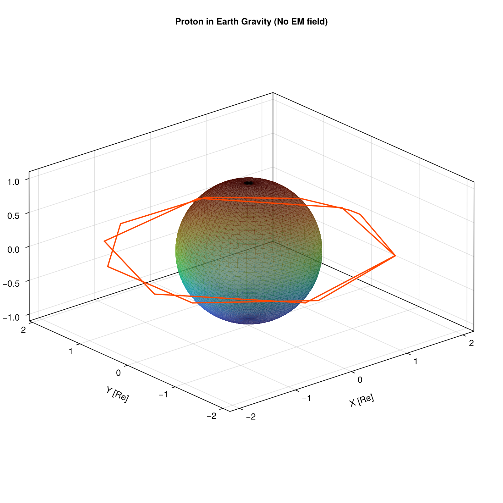
This example demonstrates tracing a proton motion with only an Earth-like gravity field provided in the external field F.

julia

using TestParticle
using OrdinaryDiffEqVerner
using StaticArrays
using LinearAlgebra
using CairoMakie

# Constants
const G = 6.67430e-11 # [m^3 kg^-1 s^-2]
const M = 5.972e24    # [kg]
const Rₑ = TestParticle.Rₑ

# Analytic fields
B(x) = SA[0.0, 0.0, 0.0]
E(x) = SA[0.0, 0.0, 0.0]

# Earth's gravity
function F(x)
   r = SA[x[1], x[2], x[3]]
   rmag = @views norm(r)
   return -G * M * TestParticle.mᵢ / rmag^3 * r
end

# Initial static particle
# Start with a location in the equatorial plane and circular motion-like velocity.
r0 = 2Rₑ
v0 = sqrt(G * M / r0)
stateinit = let x0 = [r0, 0.0, 0.0], v0 = [0.0, v0, 0.0]
   [x0..., v0...]
end

# Time span
# Orbital period T = 2π * sqrt(r^3 / GM)
T_orbit = 2π * sqrt(r0^3 / (G * M))
tspan = (0, 2T_orbit)

param = prepare(E, B, F, species = Proton)
prob = ODEProblem(trace!, stateinit, tspan, param)
# High accuracy is needed for conservation of energy and angular momentum over long periods,
# though for 2 orbits default tolerances might be acceptable.
sol = solve(prob, Vern9())

# Visualization
f = Figure(size = (800, 800))
ax = Axis3(f[1, 1],
   title = "Proton in Earth Gravity (No EM field)",
   xlabel = "X [Re]", ylabel = "Y [Re]", zlabel = "Z [Re]",
   aspect = :data
)

# Draw Earth
# A simple sphere at the origin
u = LinRange(0, 2π, 50)
v = LinRange(0, π, 50)
x_sphere = Rₑ .* (cos.(u) * sin.(v)')
y_sphere = Rₑ .* (sin.(u) * sin.(v)')
z_sphere = Rₑ .* (ones(length(u)) * cos.(v)')

surface!(ax, x_sphere ./ Rₑ, y_sphere ./ Rₑ, z_sphere ./ Rₑ,
   colormap = (:turbo, 0.5), shading = true, transparency = true)

# Plot trajectory
lines!(ax, sol[1, :] ./ Rₑ, sol[2, :] ./ Rₑ, sol[3, :] ./ Rₑ,
   color = :orangered, linewidth = 2, label = "Trajectory")

If we use lines!(ax, sol, idxs=(1,2,3)), interpolation will automatically be used. However, there is currently a bug in Makie for scale! on the axis.

Earth Gravity ​

Earth Gravity