Particle Flux

This demo shows how to estimate particle flux using TestParticle.jl. For the flux estimation to be accurate, we need to guarantee that

1. The number of test particles is sufficient to avoid statistical errors.

2. The source is properly selected. For instance, we usually sample from plasma moments of a known density, velocity and pressure. $n\cdot U$ gives us the source flux in units of [particles / s / m²]. If our source plane does not include all the possible sources, we will underestimate the target flux. Therefore, we need to make sure that our source plane covers all the launching possibilities, e.g. a closed sphere.

Under the steady state assumption, we can simulate a representative set of $N$ particles launched simultaneously. If the total physical source rate is $R$ [particles / s], each simulated particle represents a contribution of $w=R/N$ [particles / s].

The target flux (rate) is then estimated as

$$J=\sum _{i=1}^{h}w=h\cdot \frac{R}{N}$$

where $h$ is the number of particles that impact the target.

The flux density [particles / s / m²] is obtained by dividing $J$ by the target area.

In magnetosphere studies, to estimate the surface flux from ion precipitation, we can use a prescribed EM field to trace test particles originating from a closed source sphere. After a sufficiently long tracing time, each particle will either impact the surface or not.

using TestParticle, OrdinaryDiffEqTsit5, StaticArrays, Meshes, Random
import TestParticle as TP
using Meshes: Point, Plane, Sphere, Vec
using VelocityDistributionFunctions, SpecialFunctions, CairoMakie
import DisplayAs

# Source flux at the origin
const source_flux = 100.0 # [real particle / s]
const n_particles = 1000 # number of test particles
const weights = source_flux / n_particles # [particles / s per test particle]

zeroB(x) = SA[0.0, 0.0, 0.0]
zeroE(x) = SA[0.0, 0.0, 0.0]

param = prepare(zeroE, zeroB)
stateinit = zeros(6) # particle position and velocity to be modified
tspan = (0.0, 110.0) # Give particles enough time to reach the plane (x=100 with v>=1)
prob = ODEProblem(trace!, stateinit, tspan, param)

ODEProblem with uType Vector{Float64} and tType Float64. In-place: true
Non-trivial mass matrix: false
timespan: (0.0, 110.0)
u0: 6-element Vector{Float64}:
 0.0
 0.0
 0.0
 0.0
 0.0
 0.0

Flux through a Plane

In this example, we assume zero EM fields with constant particle velocities along the x-direction. We estimate the particle flux through a plane at x = 100. The estimated particle flux shall match the source flux in this example.

"""
Set initial conditions.
"""
function prob_func(prob, i, repeat)
    # initial velocity, [m/s]
    # 50% v=1.0, 50% v=2.0
    if i % 2 == 1
        v₀ = [1.0, 0.0, 0.0]
    else
        v₀ = [2.0, 0.0, 0.0]
    end
    # initial position, [m]
    r₀ = prob.u0[1:3]

    return prob = remake(prob; u0 = [r₀..., v₀...])
end

ensemble_prob = EnsembleProblem(prob; prob_func, safetycopy = false)
sols = solve(ensemble_prob, Tsit5(), EnsembleSerial(); trajectories = n_particles)

plane_loc = 100.0 # [m]
detector = Plane(Point(plane_loc, 0.0, 0.0), Vec(1.0, 0.0, 0.0))
_, weights1 = get_particle_crossings(sols, detector, weights)
flux = sum(weights1)

println("Example 1:")
println("Particle flux through plane x = $plane_loc [m]: ", flux, " /s")

Example 1:
Particle flux through plane x = 100.0 [m]: 99.99999999999987 /s

Flux through a Sphere

The second case assumes a point source at the origin. Particles are constantly isotropically launched from the source with unit speed. We estimate the particle flux through a sphere at radius r.

function prob_func_iso(prob, i, repeat)
    # initial velocity, [m/s]
    v₀ = sample_unit_sphere()
    # initial position, [m]
    r₀ = @view prob.u0[1:3]

    return prob = remake(prob; u0 = [r₀..., v₀...])
end

ensemble_prob_iso = EnsembleProblem(prob; prob_func = prob_func_iso, safetycopy = false)
sols_iso = solve(ensemble_prob_iso, Tsit5(), EnsembleSerial(); trajectories = n_particles)

r0 = 100.0 # [m]
detector_iso = Sphere(Point(0.0, 0.0, 0.0), r0)
flux, _ = get_particle_fluxes(sols_iso, detector_iso, weights)

r = 100.0 # [m]
println("Example 2:")
println("Particle flux through sphere r = $r [m]: ", flux * area(detector_iso).val, " /s")
println("Particle flux density through sphere r = $r [m]: ", flux, " /(s * m²)")

Example 2:
Particle flux through sphere r = 100.0 [m]: 99.99999999999858 /s
Particle flux density through sphere r = 100.0 [m]: 0.0007957747154594653 /(s * m²)

Multiple Detector Flux

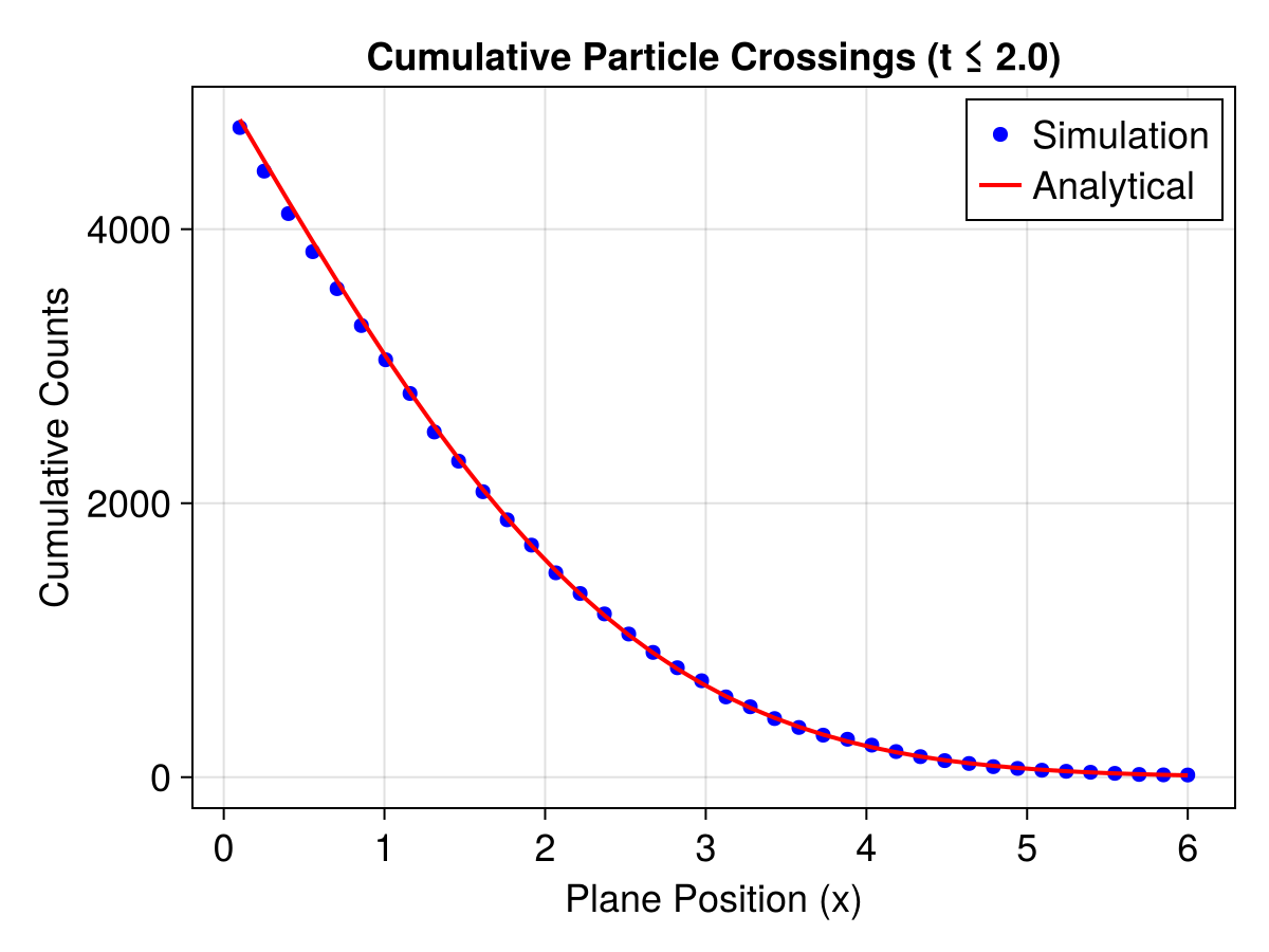
The third case demonstrates how to calculate the particle flux across multiple detectors (planes) and compares the results with the analytical solution for a freely expanding Maxwellian cloud.

Random.seed!(1234);

# Simulation Setup
N_cloud = 10_000
m = 1.0
q = 1.0
T_cloud = 1.0
# Thermal velocity: vₜₕ = sqrt(2 k_B T/m)
vth = sqrt(2 * T_cloud / m)
t_end_cloud = 2.0

# Initialize particles
# Point source at origin: r₀ = 0
x0_cloud = [SVector(0.0, 0.0, 0.0) for _ in 1:N_cloud];

# Maxwellian velocity distribution
# u_bulk = 0, n=1 effectively for distribution shape
vdf_cloud = TP.Maxwellian([0.0, 0.0, 0.0], T_cloud, 1.0; m = m)
v0_cloud = rand(vdf_cloud, N_cloud);

# Create TraceProblem template
prob_func_cloud(prob, i, repeat) = remake(prob, u0 = vcat(x0_cloud[i], v0_cloud[i]))

# Define a single problem template
param_cloud = prepare(TestParticle.ZeroField(), TestParticle.ZeroField(); q, m)
tspan_cloud = (0.0, t_end_cloud)
prob_template = ODEProblem(trace, vcat(x0_cloud[1], v0_cloud[1]), tspan_cloud, param_cloud);

ensemble_prob_cloud = EnsembleProblem(prob_template; prob_func = prob_func_cloud)
sols_cloud = solve(ensemble_prob_cloud, Tsit5(), EnsembleThreads(), trajectories = N_cloud);

# Flux Calculation with Multiple Detectors
L = 6.0
num_planes = 40
xs = range(0.1, L, length = num_planes)
detectors = [Plane(Point(x, 0.0, 0.0), Vec(1.0, 0.0, 0.0)) for x in xs]

# To match the analytical solution which is a count (not density),
# we use the raw crossing weights sum.
_, weights_cloud = get_particle_crossings(sols_cloud, detectors, 1.0);
n_crossings = [sum(w) for w in weights_cloud]

# Analytical Solution
# Fraction of particles with v_x > v_xc in a Maxwellian distribution is:
# P(v_x > v_xc) = 0.5 * erfc(v_xc/vth)
# N_cross = 0.5 * N * erfc(x_c / (vth * t_end))

n_analytic = [N_cloud / 2 * erfc(x / (vth * t_end_cloud)) for x in xs]

# Visualization
f = Figure(fontsize = 18)
ax = Axis(
    f[1, 1],
    title = "Cumulative Particle Crossings (t ≤ $t_end_cloud)",
    xlabel = "Plane Position (x)",
    ylabel = "Cumulative Counts"
)

scatter!(ax, xs, n_crossings, label = "Simulation", color = :blue, markersize = 10)
lines!(ax, xs, n_analytic, label = "Analytical", color = :red, linewidth = 2)
axislegend(ax)