Hybrid GC-FO Solver

This example demonstrates the adaptive hybrid solver that dynamically switches between full orbit (FO) and guiding center (GC) tracing based on the local adiabaticity parameter ε = ρ_L / R_c.

We use a magnetic bottle field where the adiabaticity varies spatially: near the midplane ε is large (non-adiabatic → FO), and near the mirror points ε is small (adiabatic → GC).

julia

using TestParticle, OrdinaryDiffEq, StaticArrays
import TestParticle as TP
using LinearAlgebra, Random, Printf, Markdown
using Chairmarks, Statistics
using CairoMakie

Magnetic Bottle Configuration

The magnetic field satisfies ∇·B = 0:

B_{z} = B_{0} (1 + α z^{2}), B_{x} = - B_{0} α x z, B_{y} = - B_{0} α y z

A larger α produces stronger curvature at the midplane, which raises the adiabaticity parameter ε there.

julia

const B0 = 1.0e-4   # [T]
const α = 1.0e-2    # [m⁻²]

function bottle_B(x, t)
    Bz = B0 * (1 + α * x[3]^2)
    Bx = -B0 * α * x[1] * x[3]
    By = -B0 * α * x[2] * x[3]
    return SA[Bx, By, Bz]
end

B_field = TP.Field(bottle_B)
E_field = TP.Field((x, t) -> SA[0.0, 0.0, 0.0])

m = TP.mᵢ
q = TP.qᵢ
q2m = q / m;

Step 1: Full Orbit Reference Trace

First we trace the proton using the standard ODE solver to confirm it is trapped and bounces inside the magnetic bottle.

The proton is initialized at the midplane $(x, y, z) = (0, 0, 0)$ with a perpendicular velocity $v_{⊥} = 5 \times 10^{4} m / s$ in the $x$ -direction and a parallel velocity $v_{∥} = 1 \times 10^{5} m / s$ in the $z$ -direction. This gives a significant perpendicular component needed for the mirror force to reflect the particle.

julia

x0 = SA[0.0, 0.0, 0.0]
v_perp = 5.0e4  # [m/s]
v_par = 1.0e5   # [m/s]
v0 = SA[v_perp, 0.0, v_par]
u0 = vcat(x0, v0)

Ω = abs(q2m) * B0
T_gyro = 2π / Ω

# Trace long enough to see several bounces
tspan = (0.0, 30 * T_gyro)

param_fo = prepare(E_field, B_field; species = Proton)
prob_fo = ODEProblem(trace, u0, tspan, param_fo)
sol_fo = solve(prob_fo, Vern6())

# Verify trapping: z should oscillate, not diverge
z_fo = [u[3] for u in sol_fo.u]
@assert maximum(abs, z_fo) < 1.0e4 "Particle escaped the bottle!"

Step 2: Guiding Center Reference Trace

For comparison, we also trace with the guiding center equations.

julia

bottle_B_static(x) = bottle_B(x, 0.0)
bottle_E_static(x) = SA[0.0, 0.0, 0.0]

stateinit_gc, param_gc = TP.prepare_gc(
    u0, bottle_E_static, bottle_B_static; species = Proton
)
prob_gc = ODEProblem(trace_gc!, stateinit_gc, tspan, param_gc)
sol_gc = solve(prob_gc, Vern6());

Step 3: Hybrid Solver

The adaptive hybrid solver switches between FO and GC based on the adiabaticity parameter and a threshold.

julia

# The classical adiabaticity criterion: ε = ρ_L / R_c < 0.1
threshold = 0.1

p = (q2m, m, E_field, B_field, ZeroField())

alg = AdaptiveHybrid(;
    threshold,
    dtmax = T_gyro,
    dtmin = 1.0e-4 * T_gyro,
    maxiters = 500_000,
    check_interval = 100,
)

# Set verbose = true to see the dynamic switching
prob_hybrid = TraceHybridProblem(u0, tspan, p)
sol = TP.solve(prob_hybrid, alg; verbose = false, seed = 1234).u[1];

Step 4: Compute Adiabaticity

The adiabaticity parameter ε = ρ_L / R_c measures how well the guiding center approximation holds. When ε < threshold, GC is valid; when ε ≥ threshold, we need full orbit tracing.

julia

ε_fo = get_adiabaticity(sol_fo)
ε_gc = get_adiabaticity(sol_gc)
ε_hybrid = get_adiabaticity(sol)

# Common colorbar range across all solvers
ε_clamp_lo = 1.0e-3
clims = extrema(log10.(clamp.(vcat(ε_fo, ε_gc, ε_hybrid), ε_clamp_lo, Inf)))

(-3.0, 0.21896017189514286)

Visualization

We define a helper to plot a 3D trajectory colored by ε, with start/end markers and a colorbar.

julia

# Plot a 3D trajectory colored by ε onto an existing Axis3
# When `npts` is set, the solution is interpolated for a smoother curve.
function plot_trajectory!(ax, sol, ε_vals; npts = nothing)
    if isnothing(npts)
        xs = [u[1] for u in sol.u]
        ys = [u[2] for u in sol.u]
        zs = [u[3] for u in sol.u]
        ε_plot = ε_vals
    else
        t_new = range(sol.t[1], sol.t[end]; length = npts)
        xs = Vector{Float64}(undef, npts)
        ys = Vector{Float64}(undef, npts)
        zs = Vector{Float64}(undef, npts)
        ε_plot = Vector{Float64}(undef, npts)
        for (i, t) in enumerate(t_new)
            u = sol(t)
            xs[i], ys[i], zs[i] = u[1], u[2], u[3]
            # Linearly interpolate ε to the new time grid
            idx = clamp(searchsortedlast(sol.t, t), 1, length(sol.t) - 1)
            frac = (t - sol.t[idx]) / (sol.t[idx + 1] - sol.t[idx])
            ε_plot[i] = ε_vals[idx] + frac * (ε_vals[idx + 1] - ε_vals[idx])
        end
    end
    ε_log = log10.(clamp.(ε_plot, ε_clamp_lo, Inf))
    lines!(
        ax, xs, ys, zs;
        color = ε_log, colormap = :turbo, colorrange = clims, linewidth = 1.0
    )
    scatter!(ax, [Point3f(xs[1], ys[1], zs[1])]; color = :purple, markersize = 12)
    return scatter!(
        ax, [Point3f(xs[end], ys[end], zs[end])];
        color = :red, marker = :rect, markersize = 12
    )
end

# Create a standalone figure with a 3D trajectory colored by ε
function plot_trajectory(sol, ε_vals, title_str; figsize = (700, 500), npts = nothing)
    f = Figure(; size = figsize, fontsize = 18)
    ax = Axis3(
        f[1, 1],
        xlabel = "x [m]", ylabel = "y [m]", zlabel = "z [m]",
        title = title_str, aspect = :data,
    )
    plot_trajectory!(ax, sol, ε_vals; npts)
    Colorbar(f[1, 2]; colormap = :turbo, limits = clims, label = L"\log_{10}(\epsilon)")
    return f
end

f = Figure(; size = (1400, 900), fontsize = 18)

# Compute shared axis limits from all three trajectories
lims = let
    xs = (Inf, -Inf)
    ys = (Inf, -Inf)
    zs = (Inf, -Inf)
    for sol_curr in (sol_fo, sol_gc, sol)
        for u in sol_curr.u
            xs = (min(xs[1], u[1]), max(xs[2], u[1]))
            ys = (min(ys[1], u[2]), max(ys[2], u[2]))
            zs = (min(zs[1], u[3]), max(zs[2], u[3]))
        end
    end
    (xs, ys, zs)
end

# Top row: three 3D trajectories + shared colorbar
ax_fo = Axis3(
    f[1, 1],
    xlabel = "x [m]", ylabel = "y [m]", zlabel = "z [m]",
    title = "Full Orbit", aspect = :data,
    limits = lims,
)
plot_trajectory!(ax_fo, sol_fo, ε_fo; npts = 5000)

ax_gc = Axis3(
    f[1, 2],
    xlabel = "x [m]", ylabel = "y [m]", zlabel = "z [m]",
    title = "Guiding Center", aspect = :data,
    limits = lims,
)
plot_trajectory!(ax_gc, sol_gc, ε_gc; npts = 5000)

ax_hyb = Axis3(
    f[1, 3],
    xlabel = "x [m]", ylabel = "y [m]", zlabel = "z [m]",
    title = "Hybrid Mode", aspect = :data,
    limits = lims,
)
plot_trajectory!(ax_hyb, sol, ε_hybrid)

Colorbar(f[1, 4]; colormap = :turbo, limits = clims, label = L"\log_{10}(\epsilon)")

# Bottom row: time series of adiabaticity with solver mode
t_norm = sol.t ./ T_gyro

ax_ts = Axis(
    f[2, 1:4],
    xlabel = L"t / T_\text{gyro}",
    ylabel = L"\epsilon = \rho_L / R_c",
    yscale = log10,
    title = "Adiabaticity & Solver Mode",
    limits = (
        (minimum(t_norm), maximum(t_norm)),
        (ε_clamp_lo, 10^ceil(log10(maximum(ε_hybrid)))),
    ),
)

# Shade FO and GC regions
is_fo = ε_hybrid .>= threshold
let i_region = 1
    while i_region <= length(t_norm)
        mode_fo = is_fo[i_region]
        j_region = i_region
        while j_region < length(t_norm) && is_fo[j_region + 1] == mode_fo
            j_region += 1
        end
        t_lo = t_norm[i_region]
        t_hi = t_norm[j_region]
        if mode_fo
            vspan!(ax_ts, t_lo, t_hi; color = (:red, 0.2))
        else
            vspan!(ax_ts, t_lo, t_hi; color = (:blue, 0.2))
        end
        i_region = j_region + 1
    end
end

lines!(ax_ts, t_norm, ε_hybrid; color = :black, linewidth = 1.0)
hlines!(
    ax_ts, [threshold];
    color = :gray50, linestyle = :dash, linewidth = 1.5,
    label = "threshold = $(round(threshold; sigdigits = 2))"
)

# Legend entries for solver modes
poly!(
    ax_ts, Point2f[(NaN, NaN)];
    color = (:red, 0.4), strokewidth = 0, label = "Full Orbit"
)
poly!(
    ax_ts, Point2f[(NaN, NaN)];
    color = (:blue, 0.4), strokewidth = 0,
    label = "Guiding Center"
)
Legend(f[3, 1:4], ax_ts; orientation = :horizontal)

rowsize!(f.layout, 1, Relative(0.55))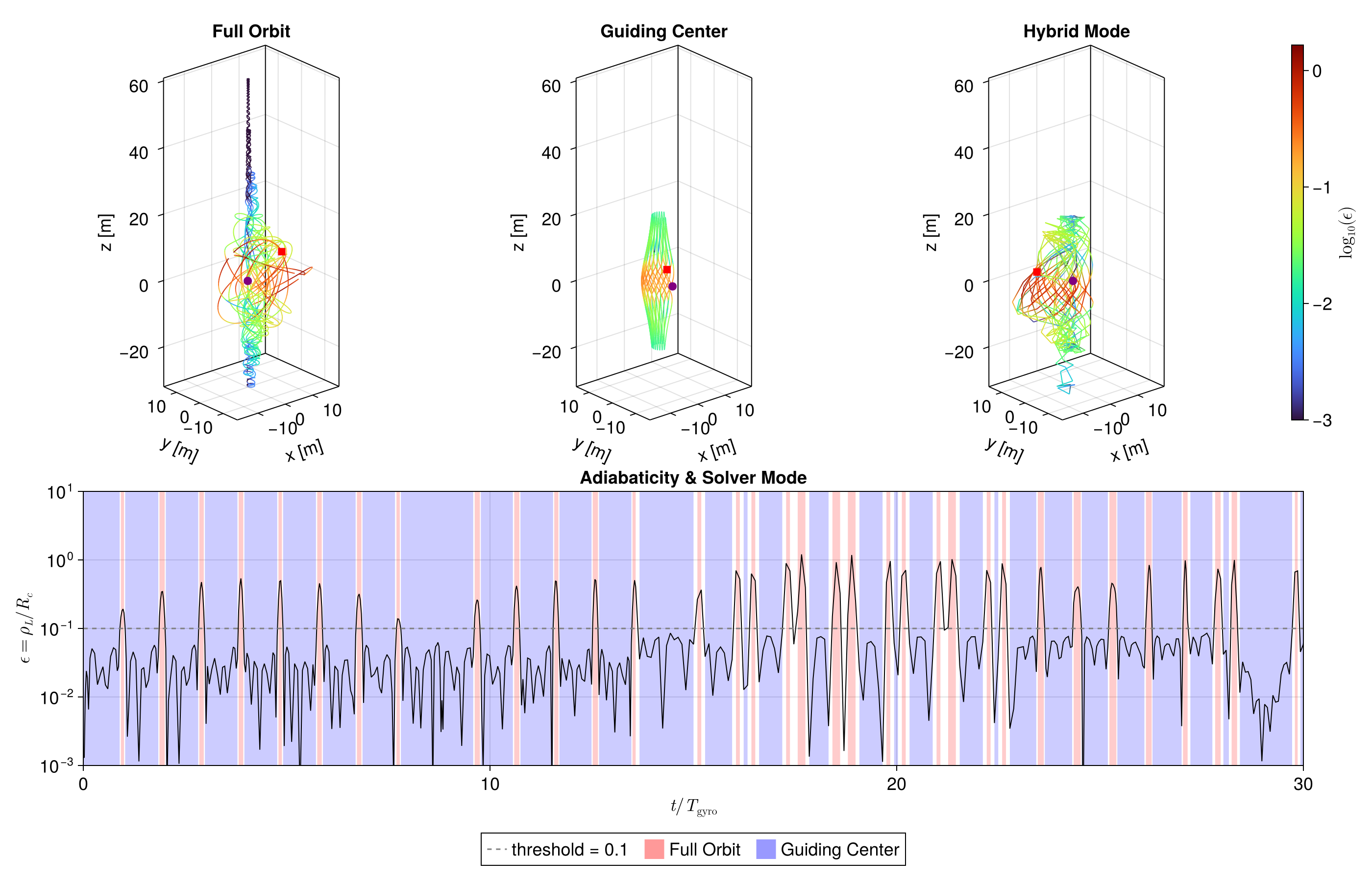

Performance Comparison

Finally, we compare the execution time and memory allocations of the three solvers.

julia

b_fo = @be solve(prob_fo, Vern6())
b_gc = @be solve(prob_gc, Vern6())
b_hy = @be TP.solve(prob_hybrid, alg; verbose = false)

Printf.@printf(
    io, "| Full Orbit | %.2f μs | %.2f KiB |\n",
    median(b_fo).time * 1.0e6, median(b_fo).bytes / 1024
Printf.@printf(
    io, "| Guiding Center | %.2f μs | %.2f KiB |\n",
    median(b_gc).time * 1.0e6, median(b_gc).bytes / 1024
Printf.@printf(
    io, "| Hybrid | %.2f μs | %.2f KiB |\n",
    median(b_hy).time * 1.0e6, median(b_hy).bytes / 1024

Solver	Time	Allocations
Full Orbit	385.32 μs	681.85 KiB
Guiding Center	392.17 μs	341.51 KiB
Hybrid	385.99 μs	58.23 KiB

AdaptiveHybrid: Adiabaticity Check Modes

AdaptiveHybrid lets the user pick which adiabaticity criterion drives the GC ↔ FO decision, via the adiabaticity keyword:

:curvature (default) → ε_curv = ρ_L / R_c (curvature drift; reproduces the legacy behaviour),
:gradB → ε_gradB = ρ_L / L_B, with L_B = |B| / |∇B|,
:both → OR of the two criteria: switch to full orbit whenever either ε_curv ≥ α or ε_gradB ≥ α (equivalently max(ε_curv, ε_gradB) ≥ α),
:jacobian → ε_jac = ρ_L · ‖JB‖_F / |B|, all-in-one criterion, which also captures torsion and shear.

All three solve the same problem; they differ only in when the solver drops into the full-orbit mode, so the trajectories stay close while the time spent in each mode changes.

julia

mode_threshold = 0.1
mode_common = (;
    threshold = mode_threshold, dtmax = T_gyro,
    dtmin = 1.0e-4 * T_gyro, maxiters = 500_000, check_interval = 100,
)
alg_curv = AdaptiveHybrid(; mode_common..., adiabaticity = :curvature)
alg_gradB = AdaptiveHybrid(; mode_common..., adiabaticity = :gradB)
alg_both = AdaptiveHybrid(; mode_common..., adiabaticity = :both)

prob_mode = TraceHybridProblem(u0, tspan, p)
sol_curv = TP.solve(prob_mode, alg_curv; verbose = false, seed = 1234).u[1]
sol_gradB = TP.solve(prob_mode, alg_gradB; verbose = false, seed = 1234).u[1]
sol_both = TP.solve(prob_mode, alg_both; verbose = false, seed = 1234).u[1]

retcode: Success
Interpolation: 1st order linear
t: 1031-element Vector{Float64}:
 0.0
 1.5317606227498457e-5
 3.070011681258181e-5
 4.885466314915151e-5
 6.538042610415581e-5
 8.455055439347887e-5
 0.00010808518255909733
 0.00013975637647483307
 0.0001834100813407995
 0.00022839425141989118
 ⋮
 0.01923045116987004
 0.019249476794971437
 0.019273499904907888
 0.019309514865209848
 0.019356223583917767
 0.019412352750013767
 0.01948992109143885
 0.019597381794291498
 0.019678342460576908
u: 1031-element Vector{StaticArraysCore.SVector{6, Float64}}:
 [0.0, 0.0, 0.0, 50000.0, 0.0, 100000.0]
 [-0.01518647543560514, -0.020816208869505637, 1.1326054935411374, 51248.71827074102, -7.968906554259775, 99365.83329959138]
 [0.1871747207543597, -0.13002128095992482, 2.3612859655969665, 53605.37754644942, -2914.4380355127214, 98071.24746608084]
 [0.759631495334792, -0.47468026802770247, 3.9703259570894875, 54212.96766092495, -11393.009712852057, 97114.1261396027]
 [1.4359467994884607, -1.0204980076122903, 5.5646387614122395, 50232.125680864934, -23036.892168631122, 97190.71545867126]
 [2.16173765388421, -1.9275736542361752, 7.511069238618554, 37756.148712685055, -39178.01044095536, 97670.65451640173]
 [2.569572309052999, -3.37043854345953, 9.923293458858438, 7896.437137189802, -55871.512543941295, 96519.53372196683]
 [1.5791013645475807, -5.335025900677888, 12.930526178190417, -52937.88077882418, -46506.910340007096, 86802.58093299661]
 [-2.173606998178864, -4.972485355211118, 15.996103094052218, -73147.3994813239, 63664.728405922324, 55644.0457827693]
 [-1.8670869572408544, -0.514295146968184, 17.828068588327604, 82654.22948566188, 66846.30814371559, 34638.82681767676]
 ⋮
 [-0.4127186484882605, 0.8091289579803094, -7.608845085720682, -22804.878698975765, -12899.118468243236, -108690.02010837672]
 [-0.9423566838834079, 0.8074798590494912, -9.713576650844471, -23629.53598900183, -2191.5214756952537, -109255.72059985013]
 [-1.5001117558592119, 1.1368505555791424, -12.380405930563587, -16097.17839873222, 15420.035377244247, -109558.53950589204]
 [-1.3345893988053579, 2.1903865117939736, -16.30501517564261, 24279.77249772833, 23035.692844477497, -106676.23786070153]
 [0.44661355693768645, 1.3265532817591543, -21.065616128180064, 5148.0684280383375, -50714.05793790557, -99506.5421382319]
 [-0.6778889991295167, 1.67912574319344, -26.679113379527834, 52177.4447798529, 20012.708627303102, -96834.78682266668]
 [0.015247034972007245, 0.3441447064216414, -33.80262426452396, -56089.69143538255, -41757.04711375006, -87236.83639788328]
 [-0.30509238473212685, 0.1924176486430611, -42.404737554824905, -84999.78698135889, 6346.96237314393, -72351.37724554281]
 [-0.08543035886116826, 0.1985415027556922, -47.65270743043339, -88995.22136393015, -35505.41341933401, -57612.37360822172]

RMS position error vs the full-orbit reference, and the FO-mode fraction.

julia

function _adia_rms(sol)
    errs = Float64[]
    for (t, u) in zip(sol.t, sol.u)
        u_ref = sol_fo(t)
        push!(errs, norm(u[1:3] - u_ref[1:3]))
    end
    return sqrt(mean(errs .^ 2))
end
function _adia_fo_frac(sol)
    mode = sol.stats.adiabaticity.mode
    return count(==(:FO), mode) / length(mode)
end

ε_col_curv = get_adiabaticity(sol_curv)
ε_col_gradB = get_adiabaticity(sol_gradB)
ε_col_both = get_adiabaticity(sol_both)

Printf.@printf(
    io2, "| `:curvature` | %.2f | %d | %.2e |\n",
    _adia_fo_frac(sol_curv), length(sol_curv.t), _adia_rms(sol_curv)
Printf.@printf(
    io2, "| `:gradB` | %.2f | %d | %.2e |\n",
    _adia_fo_frac(sol_gradB), length(sol_gradB.t), _adia_rms(sol_gradB)
Printf.@printf(
    io2, "| `:both` | %.2f | %d | %.2e |\n",
    _adia_fo_frac(sol_both), length(sol_both.t), _adia_rms(sol_both)

Result vs full-orbit reference

Mode	FO fraction	Saved points	RMS pos. err [m]
`:curvature`	0.27	544	2.68e+01
`:gradB`	0.50	780	2.99e+01
`:both`	0.77	1031	2.92e+01

Trajectories under the three modes

The three modes trace nearly the same path (all stay close to the full-orbit reference); they differ in when the solver drops into the full-orbit mode.

julia

f_modes = Figure(; size = (1400, 460), fontsize = 16)

lms = let
    lx = (Inf, -Inf)
    ly = (Inf, -Inf)
    lz = (Inf, -Inf)
    for s in (sol_curv, sol_gradB, sol_both)
        for u in s.u
            lx = (min(lx[1], u[1]), max(lx[2], u[1]))
            ly = (min(ly[1], u[2]), max(ly[2], u[2]))
            lz = (min(lz[1], u[3]), max(lz[2], u[3]))
        end
    end
    (lx, ly, lz)
end

ax_c = Axis3(
    f_modes[1, 1], title = ":curvature", aspect = :data, limits = lms,
    xlabel = "x [m]", ylabel = "y [m]", zlabel = "z [m]"
)
plot_trajectory!(ax_c, sol_curv, ε_col_curv)

ax_g = Axis3(
    f_modes[1, 2], title = ":gradB", aspect = :data, limits = lms,
    xlabel = "x [m]", ylabel = "y [m]", zlabel = "z [m]"
)
plot_trajectory!(ax_g, sol_gradB, ε_col_gradB)

ax_b = Axis3(
    f_modes[1, 3], title = ":both", aspect = :data, limits = lms,
    xlabel = "x [m]", ylabel = "y [m]", zlabel = "z [m]"
)
plot_trajectory!(ax_b, sol_both, ε_col_both)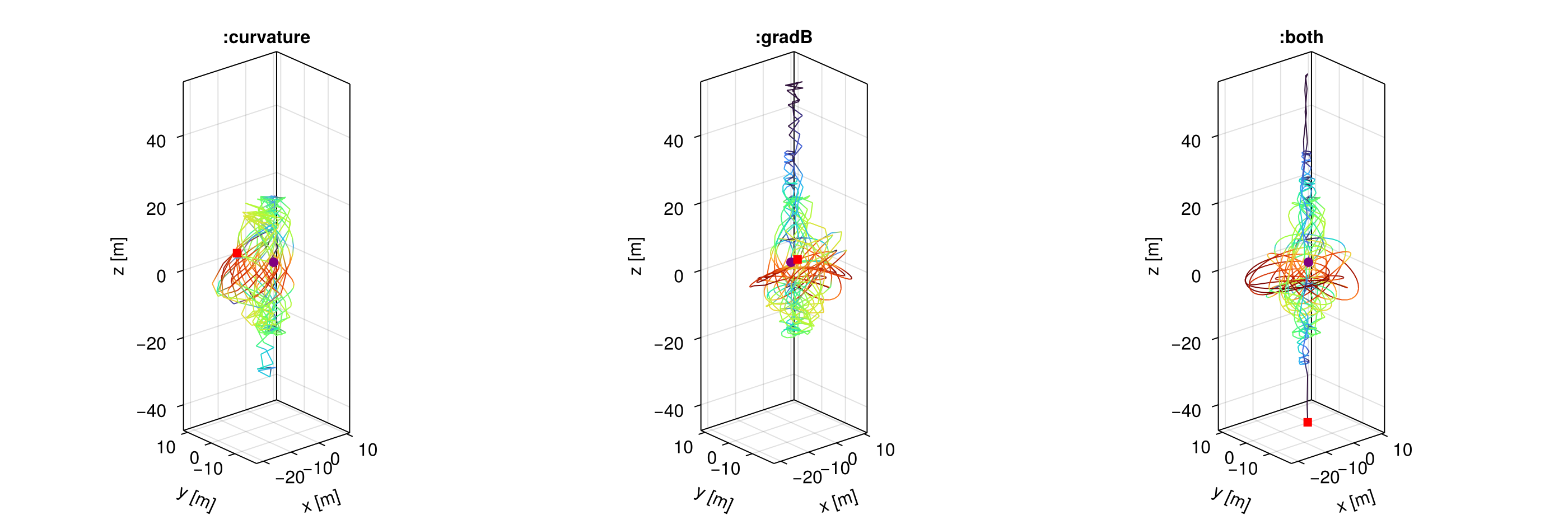

Why the modes differ: the selected adiabaticity

The diagnostics store only the adiabaticity value used by the selected mode (one scalar per check point), not the full component vector. For :curvature and :gradB that is ε_curv and ε_gradB; for :both it is max(ε_curv, ε_gradB). Plotting the stored value for each mode shows that :both switches at least as often as either single criterion alone.

julia

function _adia_traces(sol)
    t = sol.stats.adiabaticity.t ./ T_gyro
    ε = sol.stats.adiabaticity.components
    mode = sol.stats.adiabaticity.mode
    return t, ε, mode
end
t_curv, ε_curv, mode_curv = _adia_traces(sol_curv)
t_gradB, ε_gradB, mode_gradB = _adia_traces(sol_gradB)
t_both, ε_both, mode_both = _adia_traces(sol_both)

f_comp = Figure(; size = (1000, 480), fontsize = 16)
ax_comp = Axis(
    f_comp[1, 1],
    xlabel = L"t / T_\text{gyro}",
    ylabel = L"\epsilon",
    yscale = log10,
    title = "Selected adiabaticity by mode",
    limits = (
        (0.0, 30.0),
        (ε_clamp_lo, 10.0),
    ),
)

Makie.Axis with 0 plots:

Shade full-orbit (red) vs guiding-center (blue) regions for each mode.

julia

function _shade!(ax, t, mode)
    i = 1
    while i <= length(t)
        m_fo = mode[i] === :FO
        j = i
        while j < length(t) && mode[j + 1] === mode[i]
            j += 1
        end
        c = m_fo ? (:red, 0.18) : (:blue, 0.18)
        vspan!(ax, t[i], t[j]; color = c)
        i = j + 1
    end
    return
end
_shade!(ax_comp, t_curv, mode_curv)
_shade!(ax_comp, t_gradB, mode_gradB)
_shade!(ax_comp, t_both, mode_both)

lines!(ax_comp, t_curv, ε_curv; color = :green, label = ":curvature (ε_curv)")
lines!(ax_comp, t_gradB, ε_gradB; color = :orange, label = ":gradB (ε_gradB)")
lines!(ax_comp, t_both, ε_both; color = :black, linewidth = 1.6, label = ":both (max)")
hlines!(
    ax_comp, [mode_threshold];
    color = :gray50, linestyle = :dash, linewidth = 1.5,
    label = "threshold = $(round(mode_threshold; sigdigits = 2))"
)
axislegend(ax_comp; position = :rt)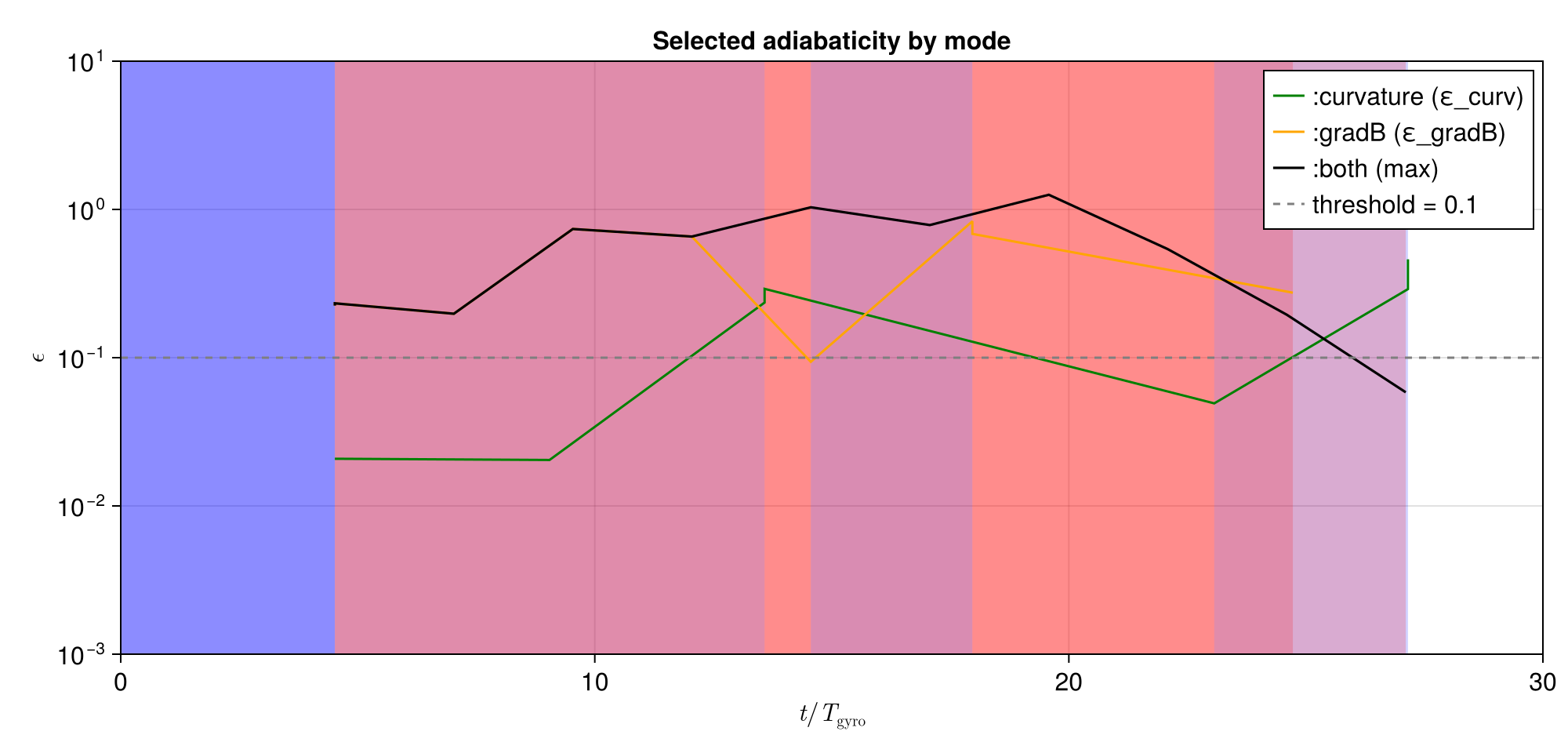

Performance

All three modes share the same solver core; :curvature carries only a few KiB of extra diagnostics. The :gradB / :both modes can even run faster in this setup because they spend more time in the cheap Boris full-orbit integrator, at the cost of higher memory (more saved points).

julia

b_curv = @be TP.solve($prob_mode, $alg_curv; verbose = false, seed = 1234)
b_gradB = @be TP.solve($prob_mode, $alg_gradB; verbose = false, seed = 1234)
b_both = @be TP.solve($prob_mode, $alg_both; verbose = false, seed = 1234)

Printf.@printf(
    io3, "| `:curvature` | %.2f ms | %.2f KiB |\n",
    median(b_curv).time * 1.0e3, median(b_curv).bytes / 1024
Printf.@printf(
    io3, "| `:gradB` | %.2f ms | %.2f KiB |\n",
    median(b_gradB).time * 1.0e3, median(b_gradB).bytes / 1024
Printf.@printf(
    io3, "| `:both` | %.2f ms | %.2f KiB |\n",
    median(b_both).time * 1.0e3, median(b_both).bytes / 1024

Mode	Time	Allocations
`:curvature`	0.31 ms	58.63 KiB
`:gradB`	0.17 ms	142.71 KiB
`:both`	0.13 ms	142.71 KiB

Hybrid GC-FO Solver ​

Magnetic Bottle Configuration ​

Step 1: Full Orbit Reference Trace ​

Step 2: Guiding Center Reference Trace ​

Step 3: Hybrid Solver ​

Step 4: Compute Adiabaticity ​

Visualization ​

Performance Comparison ​

AdaptiveHybrid: Adiabaticity Check Modes ​

Result vs full-orbit reference

Trajectories under the three modes ​

Why the modes differ: the selected adiabaticity ​

Performance ​

Hybrid GC-FO Solver

Magnetic Bottle Configuration

Step 1: Full Orbit Reference Trace

Step 2: Guiding Center Reference Trace

Step 3: Hybrid Solver

Step 4: Compute Adiabaticity

Visualization

Performance Comparison

AdaptiveHybrid: Adiabaticity Check Modes

Trajectories under the three modes

Why the modes differ: the selected adiabaticity

Performance