Tracing Magnetic Field Lines

This example demonstrates how to trace magnetic field lines in TestParticle.jl. Field line tracing is useful for visualizing the structure of magnetic fields and connecting particle trajectories to field geometry.

We will use a magnetic dipole field as a demonstration.

Setup

import TestParticle as TP
using TestParticle: trace_fieldline
using OrdinaryDiffEq
using StaticArrays
using LinearAlgebra
using CairoMakie

Define the Magnetic Field

We use the predefined dipole field functions from TestParticle. getB_dipole returns the Earth's magnetic field in SI units (Tesla).

getB = TP.getB_dipole;

Trace Field Lines

We choose a set of starting points (seeds) for the field lines. For a dipole, starting on the equatorial plane (z=0) at different radii (L-shells) is a good choice. We scale the L-shells by the Earth's radius $R_E$. Note that since trace_fieldline uses in-place operations, we need to provide mutable initial conditions (e.g., MVector).

L_shells = 3.0:1.0:6.0
seeds = [MVector(L * TP.Rₑ, 0.0, 0.0) for L in L_shells];

We trace each field line using trace_fieldline. The mode=:both argument traces in both forward (along B) and backward (against B) directions. tspan here represents the arc length to trace.

s_max = 20.0 * TP.Rₑ
s_span = (0.0, s_max);

Preallocate solutions: we expect 2 * length(seeds) solutions because mode=:both returns forward and backward traces.

solutions = Vector{ODESolution}(undef, 2 * length(seeds))

# Stop if we hit the "earth" (r < R_E)
isoutofdomain(u, p, t) = norm(u) < TP.Rₑ
callback = DiscreteCallback(isoutofdomain, terminate!)

for (i, u0) in enumerate(seeds)
   # Returns a vector of two ODEProblems (forward and backward)
   probs = trace_fieldline(u0, getB, s_span; mode = :both)

   # Solve each problem
   for (j, prob) in enumerate(probs)
      sol = solve(
         prob, Vern9(); callback, reltol = 1e-6, abstol = 1e-6, verbose = false)
      solutions[2 * (i - 1) + j] = sol
   end
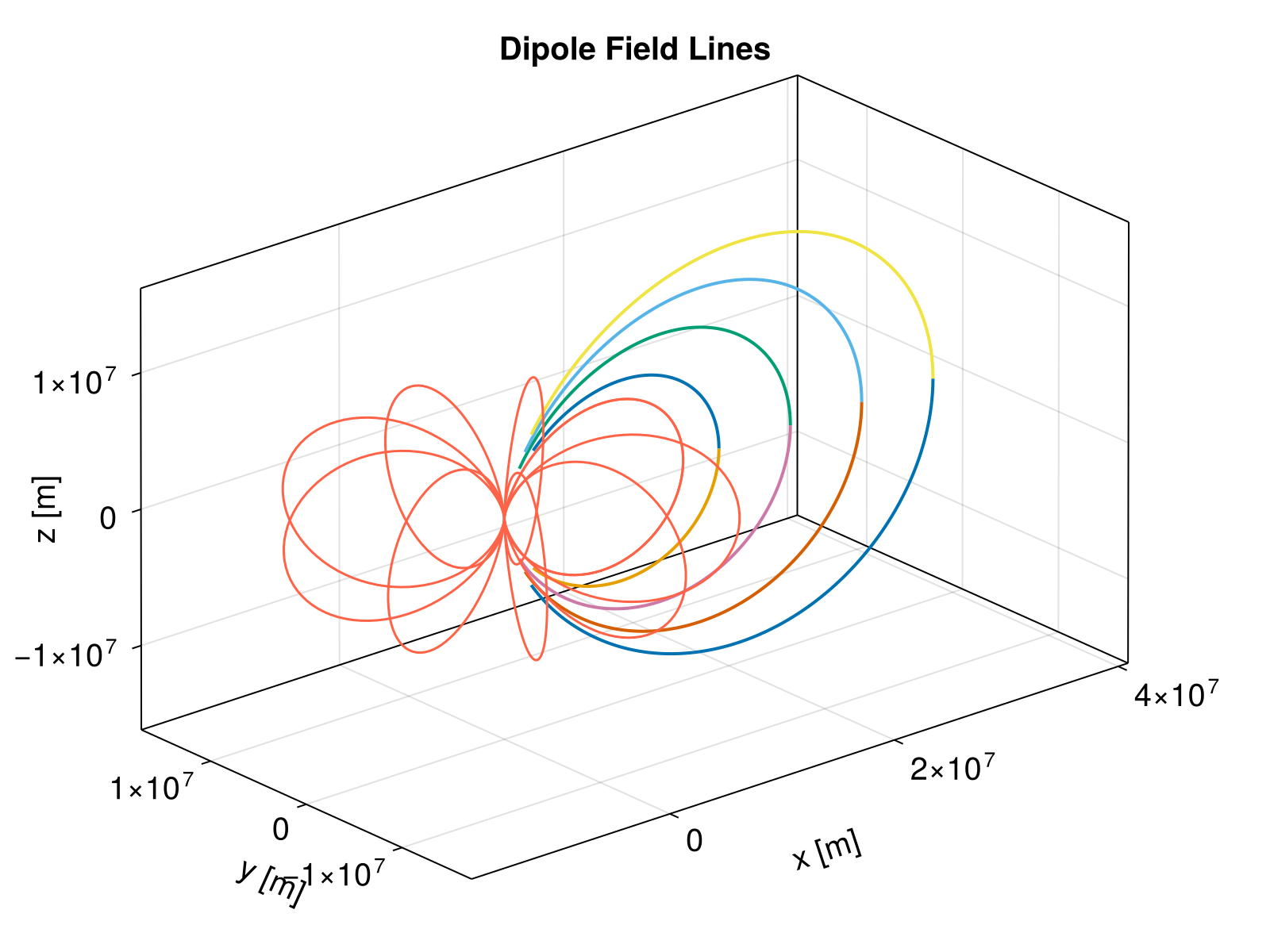
end

Visualization

We plot the traced field lines in 3D. We also overlay analytically calculated field lines for comparison.

f = Figure(size = (800, 600))
ax = Axis3(f[1, 1], aspect = :data, xlabel = "x [m]", ylabel = "y [m]",
   zlabel = "z [m]", title = "Dipole Field Lines")

# Plot traced field lines
for sol in solutions
   lines!(ax, sol; idxs = (1, 2, 3), linewidth = 2)
end

# Plot analytic field lines for reference
for ϕ in range(0, stop = 2 * π, length = 10)
   lines!(ax, TP.dipole_fieldline(ϕ) .* TP.Rₑ..., color = :tomato)
end