Shock Drift Acceleration

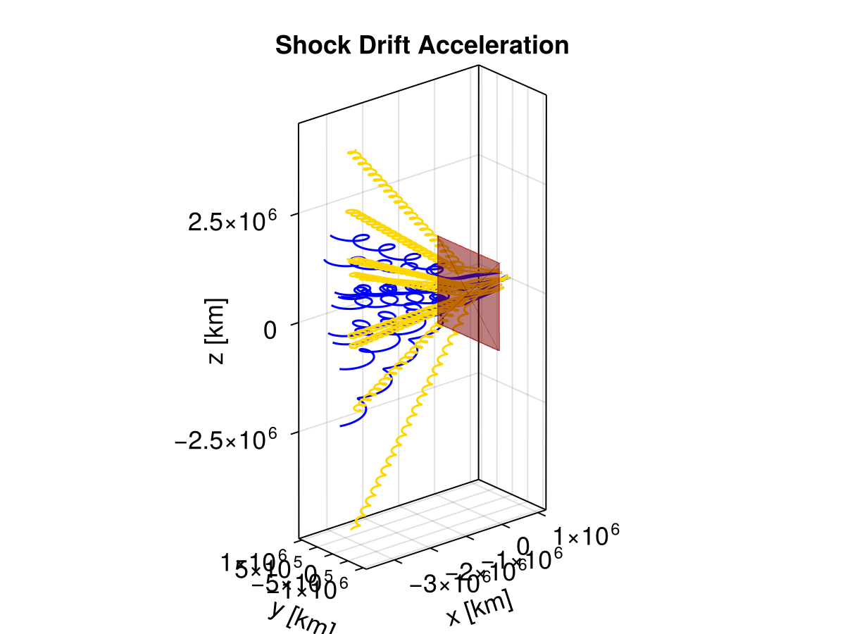
This example demonstrates Shock Drift Acceleration (SDA) where particles gain energy by drifting along the electric field at a shock front. The setup mimics the visualization NASA SVS 4513, which uses a heavy electron (mass = 1/5 proton mass) to make the gyroradii comparable for visualization purposes.

using TestParticle
using TestParticle: mᵢ, qᵢ
using OrdinaryDiffEqVerner
using LinearAlgebra
using Statistics
using CairoMakie
using Random

Random.seed!(42);

Shock Parameters

We set up a perpendicular shock. Upstream (Region 1): High velocity, Low B. Downstream (Region 2): Low velocity, High B.

n₁ = 1.0e6
V₁ = [-545.0, 0.0, 0.0] .* 1e3 # Upstream velocity (flowing left)
B₁ = [0.0, 0.0, 5.0] .* 1e-9   # Upstream B (z-direction)

V₂ = [-172.0, 0.0, 0.0] .* 1e3 # Downstream velocity
B₂ = [0.0, 0.0, 15.8] .* 1e-9; # Downstream B

Calculate Convection Electric Field E = -V x B

E₁ = cross(B₁, V₁)
E₂ = cross(B₂, V₂);

Grid Setup

We use a 1D grid in x-direction. The shock is located at x=0.

x_max = 2000e3 # 2000 km
x = range(-x_max, x_max, length = 1000) # 4000 km total, 4 km resolution

B = repeat(B₁, 1, length(x))
E = repeat(E₁, 1, length(x))

# Set downstream values (x < 0)
mid_ = findfirst(v -> v >= 0, x)
B[:, 1:(mid_ - 1)] .= B₂
E[:, 1:(mid_ - 1)] .= E₂;

E-field Bump

Add a Gaussian enhancement to the Electric field at the shock. "interaction of the two regions in the shock wave generates an increase in the electric field." We enhance the magnitude of Ey (which is negative).

bump_amp = 2.0 # Enhance by factor of 2 at peak
bump_width = 100e3 # 100 km width
for i in eachindex(x)
   # Gaussian centered at 0
   factor = 1.0 + bump_amp * exp(-(x[i] / bump_width)^2)
   E[2, i] *= factor
end

Particle Tracing

We trace Protons and "Heavy Electrons". Heavy Electron mass is set to m_p / 5 for visualization.

const m_heavy = mᵢ / 5.0
const q_heavy = -qᵢ
const v0_p = V₁
const x0 = 1000e3; # 1000 km upstream

Protons

prob_p = let
   param_p = prepare(x, E, B; species = Proton, bc = 3)
   u0_p = [x0, 0.0, 0.0, v0_p...]
   ODEProblem(trace!, u0_p, (0.0, 20.0), param_p)
end;

"""
Create ensemble of protons.
"""
function prob_func_p(prob, i, repeat)
   # Randomize y and z slightly to separate lines
   r = rand(2)
   r0 = (x0, (r[1]-0.5)*500e3, (r[2]-0.5)*500e3)
   # Small thermal spread
   v_th = 50e3 # 50 km/s
   v = v0_p .+ randn(3) .* v_th
   remake(prob; u0 = [r0..., v...])
end

ensemble_p = EnsembleProblem(prob_p; prob_func = prob_func_p)
sols_p = solve(ensemble_p, Vern9(), EnsembleSerial(); trajectories = 10);

Heavy Electrons

prob_e = let
   # Create parameter object for Heavy Electron.
   param_e = prepare(x, E, B; bc = 3, q = q_heavy, m = m_heavy)

   u0_e = [x0, 0.0, 0.0, v0_p...]
   ODEProblem(trace!, u0_e, (0.0, 20.0), param_e)
end;

function prob_func_e(prob, i, repeat)
   r0 = [x0, (rand()-0.5)*500e3, (rand()-0.5)*500e3]
   v_th = 100e3
   v = v0_p .+ randn(3) .* v_th
   remake(prob; u0 = [r0..., v...])
end

ensemble_e = EnsembleProblem(prob_e; prob_func = prob_func_e)
sols_e = solve(ensemble_e, Vern9(), EnsembleSerial(); trajectories = 10);

Visualization

f = Figure(fontsize = 18)
ax = Axis3(f[1, 1], title = "Shock Drift Acceleration", xlabel = "x [km]",
   ylabel = "y [km]", zlabel = "z [km]", aspect = :data)

# Plot Protons
for sol in sols_p
   lines!(ax, sol, idxs = (1, 2, 3), color = :blue, linewidth = 1.5)
end

# Plot Heavy Electrons
for sol in sols_e
   lines!(ax, sol, idxs = (1, 2, 3), color = :gold, linewidth = 1.5)
end

# Draw Shock Plane
mesh!(ax, Rect3f(Point3f(-10e3, -1000e3, -1000e3), Vec3f(20e3, 2000e3, 2000e3)), color = (
   :red, 0.3))