Electron in a Magnetic Bottle

This example shows how to trace non-relativistic and relativistic electrons in a stationary magnetic field that corresponds to a magnetic bottle. Reference wiki
julia
using TestParticle, OrdinaryDiffEq, StaticArrays
import TestParticle as TP
using Printf
using CairoMakie

### Obtain field

# Magnetic bottle parameters in SI units
const I1 = 20.0 # current in the solenoid
const N1 = 45 # number of windings
const I2 = 20.0 # current in the central solenoid
const N2 = 45 # number of windings
const distance = 10.0 # distance between solenoids
const a = 4.0 # radius of each coil
const b = 8.0 # radius of central coil

getB(xu) = SVector{3}(TP.getB_bottle(xu[1], xu[2], xu[3], distance, a, b, I1 * N1, I2 * N2))

### Initialize particles
m = TP.mₑ
q = TP.qₑ
c = TP.c

# initial velocity, [m/s]
v₀ = [2.75, 2.5, 1.3] .* 0.03c  # confined
# initial position, [m]
r₀ = [0.8, 0.8, 0.0]
stateinit = [r₀..., v₀...]

# Theoretically we can take advantage of the fact that magnetic field does not
# accelerate particles, so that γ remains constant. However, we are not doing
# that here since it is not generally true in the EM field.

param = prepare(TP.ZeroField(), getB; species = Electron)
tspan = (0.0, 1.0e-5)

prob_rel = ODEProblem(trace_relativistic!, stateinit, tspan, param)
prob_non = ODEProblem(trace!, stateinit, tspan, param)

vratio = √(v₀[1]^2 + v₀[2]^2 + v₀[3]^2) / c
E = (1 / √(1 - vratio^2) - 1) * m * c^2 / abs(q) / 1.0e6

v_str = @sprintf "V = %4.2f %s" vratio * 100 "% c"
e_str = @sprintf "E = %6.4f MeV" E

println(v_str)
println(e_str)

# Default Tsit5() and many solvers does not work in this case!
sol_rel = solve(prob_rel, AB4(); dt = 3.0e-9)
sol_non = solve(prob_non, AB4(); dt = 3.0e-9)

### Visualization

f = Figure(fontsize = 18)
ax1 = Axis3(
    f[1, 1];
    aspect = :data,
    title = "Relativistic e⁻, \n" * v_str * ", " * e_str
)
ax2 = Axis3(
    f[1, 2];
    aspect = :data,
    title = "Non-relativistic e⁻, \n" * v_str * ", " * e_str
)

lines!(ax1, sol_rel, idxs = (1, 2, 3))
lines!(ax2, sol_non, idxs = (1, 2, 3))

# Plot coils
θ = range(0, 2π, length = 100)
x = a .* cos.(θ)
y = a .* sin.(θ)
z = fill(distance / 2, size(x))
for ax in (f[1, 1], f[1, 2])
    lines!(ax, x, y, z, color = (:red, 0.7))
end
z = fill(-distance / 2, size(x))
for ax in (f[1, 1], f[1, 2])
    lines!(ax, x, y, z, color = (:red, 0.7))
end

x = b .* cos.(θ)
y = b .* sin.(θ)
z = fill(0.0, size(x))
for ax in (f[1, 1], f[1, 2])
    lines!(ax, x, y, z, color = (:red, 0.7))
end

using FieldTracer

xrange = range(-4, 4, length = 20)
yrange = range(-4, 4, length = 20)
zrange = range(-10, 10, length = 20)

Bx, By, Bz = let x = xrange, y = yrange, z = zrange
    Bx = zeros(length(x), length(y), length(z))
    By = zeros(length(x), length(y), length(z))
    Bz = zeros(length(x), length(y), length(z))
    for k in eachindex(z), j in eachindex(y), i in eachindex(x)
        Bx[i, j, k], By[i, j, k], Bz[i, j, k] = getB([x[i], y[j], z[k]])
    end

    Bx, By, Bz
end

for i in 0:8
    if i == 0
        xs, ys, zs = 0.0, 0.0, 0.0
    else
        xs, ys, zs = 3 * cos(2π * (i - 1) / 8), 3 * sin(2π * (i - 1) / 8), 0.0
    end
    x1, y1,
        z1 = FieldTracer.trace(
        Bx, By, Bz, xs, ys, zs, xrange, yrange, zrange;
        ds = 0.1, maxstep = 1000
    )
    for ax in (f[1, 1], f[1, 2])
        lines!(ax, x1, y1, z1, color = :black)
    end
end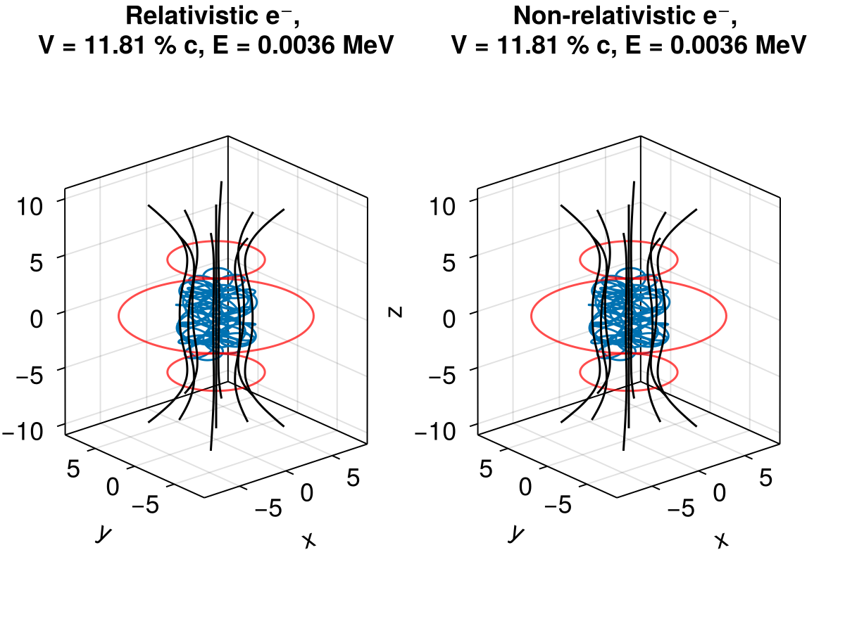
We see that at about 12% of the speed of light, relativistic effects are not significant.
Electron in a Magnetic Bottle ​

Electron in a Magnetic Bottle
