Magnetic Fields from Current Loops

This example demonstrates how to generate and visualize magnetic fields created by current loops using the Biot-Savart law. We will create two current loops with different orientations and trace the resulting magnetic field lines.

Setup

import TestParticle as TP
import Magnetostatics as MS
using OrdinaryDiffEqVerner
using StaticArrays
using LinearAlgebra
using CairoMakie

Define Current Loops

We define two current loops:

1. A primary loop in the xy-plane (normal along z-axis).

2. A tilted loop to demonstrate arbitrary orientation.

# Loop 1: Radius 1.0, Current 1.0 MA, located at origin, normal along z
R1 = [0.0, 0.0, 0.0]
a1 = 1.0
I1 = 1.0e6
n1 = [0.0, 0.0, 1.0]
loop1 = MS.CurrentLoop(a1, I1, R1, n1)

# Loop 2: Radius 0.5, Current 0.5 MA, located at [2, 0, 0], tilted 45 degrees
R2 = [2.0, 0.0, 0.0]
a2 = 0.5
I2 = 0.5e6
n2 = normalize([1.0, 0.0, 1.0])
loop2 = MS.CurrentLoop(a2, I2, R2, n2)

Magnetostatics.CurrentLoop{Float64}(0.5, 500000.0, [2.0, 0.0, 0.0], [0.7071067811865476, 0.0, 0.7071067811865476])

Define the Magnetic Field Function

The total magnetic field is the vector sum of the fields from each loop. We define a function B_total(x) that calculates this sum. getB_loop handles the Biot-Savart calculation.

function get_B_total(loop1, loop2)
    return x -> begin
        B1 = MS.getB_loop(x, loop1)
        B2 = MS.getB_loop(x, loop2)
        return B1 + B2
    end
end

B_total = get_B_total(loop1, loop2)
param = TP.prepare(TP.ZeroField(), B_total);

Trace Field Lines

We select starting points (seeds) for tracing. We'll pick points passing through the loops to visualize the field structure.

# Seeds for Loop 1
seeds1 = [MVector(x, 0.0, 0.0) for x in 0.1:0.2:0.9]
# Seeds for Loop 2 (relative to its center)
seeds2 = [MVector(R2[1] + x, R2[2], R2[3] + 0.1) for x in -0.4:0.2:0.4]

seeds = vcat(seeds1, seeds2)

s_span = (0.0, 10.0) # Trace length

solutions = Vector{ODESolution}()

# Define a domain check to stop tracing if we go too far
isoutofdomain(u, p, t) = norm(u) > 10.0
callback = DiscreteCallback(isoutofdomain, terminate!)

for u0 in seeds
    # Trace in both directions
    probs = TP.trace_fieldline(u0, param, s_span; mode = :both)

    for prob in probs
        sol = solve(
            prob, Vern9(); callback, reltol = 1.0e-6, abstol = 1.0e-6, verbose = false
        )
        push!(solutions, sol)
    end
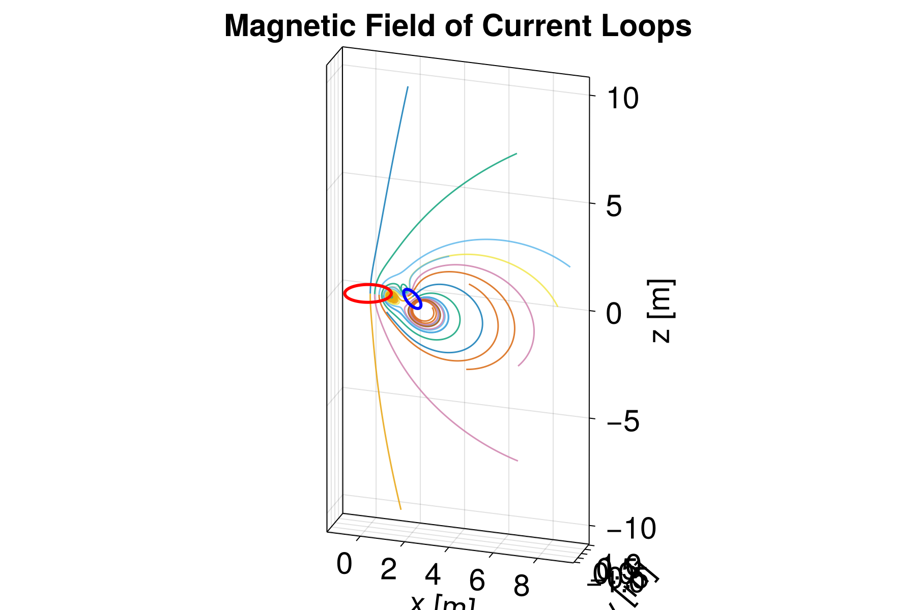
end

Visualization

We plot the field lines and the current loops.

# Helper to visualize the loops
function plot_loop!(ax, center, radius, normal, color)
    # Generate circle points in 2D
    θ = range(0, 2π, length = 100)
    x_circ = radius .* cos.(θ)
    y_circ = radius .* sin.(θ)
    z_circ = zeros(length(θ))

    points = [SVector(x, y, z) for (x, y, z) in zip(x_circ, y_circ, z_circ)]

    # Rotate to align with normal
    z_axis = [0.0, 0.0, 1.0]
    if !isapprox(normal, z_axis) && !isapprox(normal, -z_axis)
        v = cross(z_axis, normal)
        s = norm(v)
        c = dot(z_axis, normal)
        Vx = [0 -v[3] v[2]; v[3] 0 -v[1]; -v[2] v[1] 0]
        R = I + Vx + Vx^2 * (1 - c) / s^2
        points = [R * p for p in points]
    elseif isapprox(normal, -z_axis)
        points = [SVector(p[1], -p[2], -p[3]) for p in points] # simple flip
    end

    # Translate to center
    points = [p + center for p in points]

    return lines!(
        ax, [p[1] for p in points], [p[2] for p in points],
        [p[3] for p in points], color = color, linewidth = 3
    )
end

f = Figure(size = (900, 600), fontsize = 30)
ax = Axis3(
    f[1, 1], aspect = :data, azimuth = 1.6pi,
    xlabel = "x [m]", ylabel = "y [m]", zlabel = "z [m]", title = "Magnetic Field of Current Loops"
)

# Plot field lines
for sol in solutions
    lines!(ax, sol; idxs = (1, 2, 3), linewidth = 1.5, alpha = 0.8)
end

plot_loop!(ax, R1, a1, n1, :red)
plot_loop!(ax, R2, a2, n2, :blue)