Energy Conservation

This example demonstrates the energy conservation of a single particle motion in four cases. 2. Constant B field, Zero E field.

3. Constant E field, Zero B field.

4. Magnetic Mirror.

5. ExB drift in constant electric and magnetic fields.

The tests are performed in dimensionless units with q=1, m=1. We compare the following groups of solvers:

• Common solvers from OrdinaryDiffEq.

• Native Boris solvers.

• The native guiding-center (GC) solver, whose conserved Hamiltonian is $H_{GC}=\frac{1}{2}m{v}_{\parallel }^2+\mu B+q\varphi$. For $E=0$ this reduces to $E_{GC}=\frac{1}{2}m{v}_{\parallel }^2+\mu B$ and equals the full-orbit kinetic energy, so it is compared against the full-orbit reference. When $E\ne 0$ (Case 4) the GC is a gyro-averaged model whose Hamiltonian differs from the full-orbit kinetic energy by the guiding-center approximation, so it is benchmarked against its own initial $H_{GC}$.

• The native adaptive hybrid (GC <-> full-orbit) solver, whose output is the full-orbit state, so its energy is the ordinary kinetic energy.

(Note: Geometric integrators from GeometricIntegratorsDiffEq were previously included but removed due to poor performance and compatibility issues in the current environment.)

using Printf
using TestParticle
using OrdinaryDiffEq, OrdinaryDiffEqLowOrderRK, OrdinaryDiffEqSDIRK
using StaticArrays
using LinearAlgebra: ×, norm
using CairoMakie

const q = 1.0
const m = 1.0
const B₀ = 1.0
const E₀ = 1.0
const Ω = q * B₀ / m
const T = 2π / Ω

# Helper function to run tests
function run_test(
        case_name, param, x0, v0, tspan, expected_energy_func;
        uselog = true, dt = 0.1, ymin = nothing, ymax = nothing,
        odes = nothing, symplectics = nothing, natives = nothing,
        gc = false, hybrid = false, gc_phi = nothing
    )
    results = Tuple{String, Float64}[]
    u0 = [x0..., v0...]
    prob_ode = ODEProblem(trace_normalized!, u0, tspan, param)
    prob_tp = TraceProblem(u0, tspan, param)
    prob_dyn = DynamicalODEProblem(get_dv!, get_dx!, v0, x0, tspan, param)

    f = Figure(size = (1000, 600), fontsize = 18)
    if uselog
        yscale = log10
    else
        yscale = identity
    end

    ax = Axis(
        f[1, 1],
        title = "$case_name: Energy Error",
        xlabel = "Time [Gyroperiod]",
        ylabel = L"Rel. Energy Error $|(E - E_\mathrm{ref})/E_\mathrm{ref}|$",
        yscale = yscale
    )

    if !isnothing(ymin) && !isnothing(ymax)
        ylims!(ax, ymin, ymax)
    end

    color_idx = 1
    m_ = param[2]
    fo_energy(u, t) = 0.5 * m_ * norm(u[4:6])^2

    function plot_energy_error!(
            sol, label, i; energy_of = fo_energy,
            expected_of = expected_energy_func
        )
        # Calculate energy with the solver-specific extractor.
        E = [energy_of(u, ti) for (u, ti) in zip(sol.u, sol.t)]

        # Expected energy (full-orbit analytic reference). The full state `u`
        # is passed as the velocity argument; all reference functions in this
        # demo ignore it and depend only on `t` (and `x` for Case 2b).
        t = sol.t
        x = @views [u[1:3] for u in sol.u]
        E_ref = [
            expected_of(ti, xi, u)
                for (ti, xi, u) in zip(t, x, sol.u)
        ]

        # Error (Avoid division by zero if E_ref is 0)
        error = abs.(E .- E_ref) ./ (abs.(E_ref) .+ 1.0e-16)
        push!(results, (label, maximum(error)))

        return lines!(
            ax, t[1:length(error)] ./ T, error;
            label, color = i, colormap = :tab20, colorrange = (1, 20)
        )
    end

    # Run ODE solvers
    _odes = odes === nothing ? ode_solvers : odes
    for (name, alg) in _odes
        sol = solve(prob_ode, alg; adaptive = false, dt, dense = false)
        plot_energy_error!(sol, name, color_idx)
        color_idx += 1
    end


    # Run symplectic solvers
    _symplectics = symplectics === nothing ? symplectic_solvers : symplectics
    for (name, alg) in _symplectics
        sol = solve(prob_dyn, alg; dt, adaptive = false)
        plot_energy_error!(sol, name, color_idx)
        color_idx += 1
    end

    # Run native solvers
    _natives = natives === nothing ? native_solvers : natives
    for (name, alg) in _natives
        sol = TestParticle.solve(prob_tp, alg; dt).u[1]
        plot_energy_error!(sol, name, color_idx)
        color_idx += 1
    end

    # Run guiding-center (GC) solver. The GC conserves its own energy
    # E_GC = ½ m v_∥² + μ B; for static fields this equals the full-orbit
    # kinetic energy, so it is compared against the same analytic reference.
    if gc
        q2m, m_gc, Efunc, Bfunc, _ = param
        state_gc, μ_gc = full_to_gc(SVector{6}(u0...), param)
        p_gc = (q2m * m_gc, q2m, μ_gc, Efunc, Bfunc)
        prob_gc = TraceGCProblem(state_gc, tspan, p_gc)
        sol_gc = TestParticle.solve(prob_gc; dt, alg = :rk4).u[1]
        q_gc = q2m * m_gc
        function gc_energy(u, t)
            e = 0.5 * m_gc * u[4]^2 + μ_gc * norm(Bfunc(u[1:3], t))
            if !isnothing(gc_phi)
                # Include the electrostatic potential so that the GC conserves
                # its Hamiltonian H_GC = ½ m v_∥² + μ B + q φ, matching
                # full-orbit energy conservation when E ≠ 0.
                e += q_gc * gc_phi(u[1:3])
            end
            return e
        end
        # The GC conserves its Hamiltonian H_GC = ½ m v_∥² + μ B + q φ, which
        # differs from the full-orbit kinetic energy by the guiding-center
        # (gyro-averaging) approximation when E ≠ 0. For a meaningful
        # conservation check we benchmark it against its own initial value
        # rather than the full-orbit KE reference.
        gc_E0 = gc_energy(sol_gc.u[1], sol_gc.t[1])
        plot_energy_error!(
            sol_gc, "GC (RK4)", color_idx;
            energy_of = gc_energy, expected_of = (t, x, u) -> gc_E0
        )
        color_idx += 1
    end

    # Run adaptive hybrid (GC <-> full-orbit) solver. Its output is the full
    # orbit state, so its energy is the ordinary kinetic energy.
    if hybrid
        q2m, m_hy, Efunc, Bfunc, _ = param
        p_hy = (q2m, m_hy, Efunc, Bfunc, ZeroField())
        prob_hy = TraceHybridProblem(SVector{6}(u0...), tspan, p_hy)
        alg_hy = AdaptiveHybrid(;
            threshold = 0.1, dtmax = T, dtmin = 1.0e-3 * T,
            check_interval = 20, save_adiabaticity = false
        )
        sol_hy = TestParticle.solve(prob_hy, alg_hy; seed = 1234).u[1]
        plot_energy_error!(sol_hy, "Hybrid", color_idx)
        color_idx += 1
    end

    f[1, 2] = Legend(f, ax, "Solvers", framevisible = false, labelsize = 24)

    return f, results
end

function plot_table(results)
    io = IOBuffer()
    println(io, "| Solver | Max Rel. Error |")
    println(io, "| :--- | :--- |")
    for (name, err) in results
        println(io, "| $name | $(@sprintf("%.1e", err)) |")
    end
    return Markdown.parse(String(take!(io)))
end

# Solvers to test
const ode_solvers = [
    ("Tsit5", Tsit5()),
    ("Vern7", Vern7()),
    ("Vern9", Vern9()),
    ("BS3", BS3()),
    ("ImplicitMidpoint", ImplicitMidpoint()),
]

const symplectic_solvers = []

const native_solvers = [
    ("Boris", Boris()),
    ("Boris Multistep (n=2)", MultistepBoris2(; n = 2)),
    ("Hyper Boris (n=2, N=4)", MultistepBoris4(; n = 2)),
];

Case 1: Constant B, Zero E

Energy should be conserved.

uniform_B(x) = SA[0, 0, B₀]

param1 = prepare(ZeroField(), uniform_B; q = q, m = m)
x0_1 = [0.0, 0.0, 0.0]
v0_1 = [1.0, 0.0, 0.0]
tspan1 = (0.0, 50.0)
E_func1(t, x, v) = 0.5 * m * norm(v0_1)^2 # Constant energy

f, results = run_test(
    "Constant B", param1, x0_1, v0_1, tspan1, E_func1;
    dt = T / 4, ymin = 1.0e-16, ymax = 2.0, gc = true, hybrid = true
)

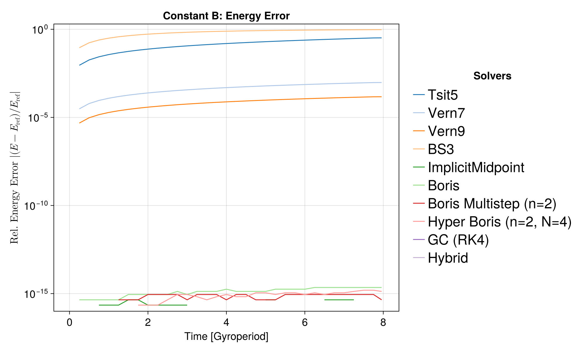
Solver comparisons:

Solver	Max Rel. Error
Tsit5	3.3e-01
Vern7	9.6e-04
Vern9	1.5e-04
BS3	9.5e-01
ImplicitMidpoint	4.4e-16
Boris	2.2e-15
Boris Multistep (n=2)	8.9e-16
Hyper Boris (n=2, N=4)	1.6e-15
GC (RK4)	0.0e+00
Hybrid	0.0e+00

Case 2a: Linear E(t), Zero B

Energy increases due to work done by the electric field which grows linearly in time. For a particle starting from rest in an electric field $\mathbf{E}(t)=E_{0}t$:

$$\begin{array}{rl}\mathbf{E}(t)& =E_{0}t\\ \mathbf{a}(t)& =\frac{q{E}_0}{m}t\\ \mathbf{v}(t)& =\frac{q{E}_0}{2m}{t}^2(\mathrm{if}{v}_0=0)\end{array}$$$$E_{kin}=\frac{1}{2}m{v}^2=\frac{q^2{E}_0^2}{8m}{t}^4$$

linear_E(x, t) = SA[E₀ * t, 0.0, 0.0]

param2a = prepare(linear_E, ZeroField(); q = q, m = m)
x0_2a = [0.0, 0.0, 0.0]
v0_2a = [0.0, 0.0, 0.0] # Start from rest
tspan2a = (0.0, 40.0)

function E_func2a(t, x, v)
    v_theo = (q * E₀ / m) * (t^2 / 2) # analytical energy
    return 0.5 * m * v_theo^2
end

f, results = run_test(
    "Linear E(t)", param2a, x0_2a, v0_2a, tspan2a,
    E_func2a; dt = T / 4, ymin = 1.0e-16, ymax = 1.0e4, hybrid = true
)

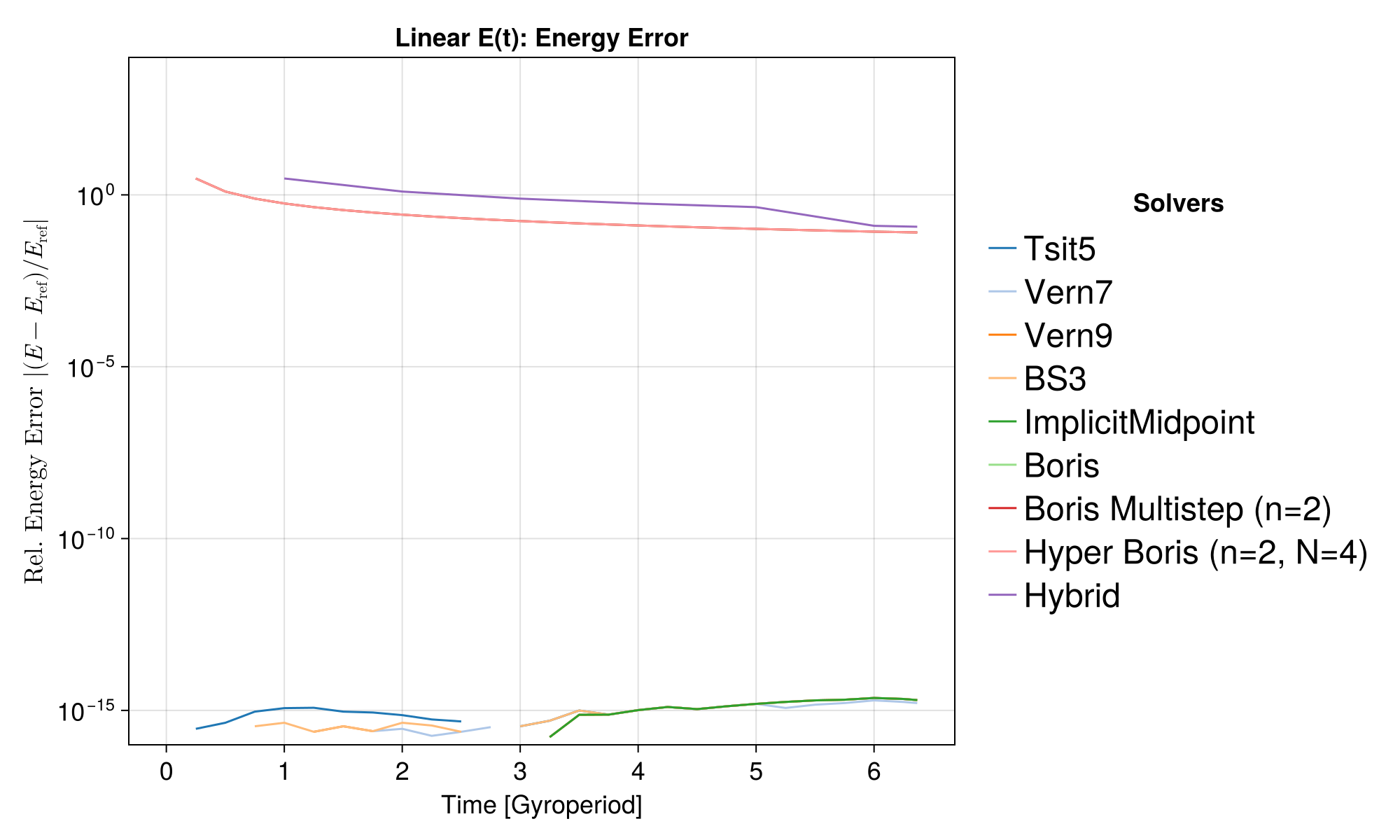
Solver comparisons:

Solver	Max Rel. Error
Tsit5	2.3e-15
Vern7	2.0e-15
Vern9	2.3e-15
BS3	2.3e-15
ImplicitMidpoint	2.3e-15
Boris	3.0e+00
Boris Multistep (n=2)	3.0e+00
Hyper Boris (n=2, N=4)	3.0e+00
Hybrid	3.0e+00

The Boris solvers systematically show a large error in this case. This is because Boris evaluates the electric field at the integer time step $t_n$ to update the velocity from $v_{n-1/2}$ to $v_{n+1/2}$ (in its standard leapfrog staggered form), while the current implementation evaluates at $t_{n+1/2}$, leading to an offset for time-varying fields. The Boris solvers systematically show a large error in this case, because of the initial half-step offset.

Case 2b: Spatially Linear E(x), Zero B

Here we test energy conservation in a spatially varying electric field $\mathbf{E}(x)=E_{0}x\hat{x}$. The total energy $H=\frac{1}{2}m{v}^2+q\mathrm{\Phi }(x)$ is conserved, where $\mathrm{\Phi }(x)=-\frac{1}{2}{E}_0{x}^2$.

spatial_linear_E(x, t) = SA[E₀ * x[1], 0.0, 0.0]

param2b = prepare(spatial_linear_E, ZeroField(); q = q, m = m)
# Set an initial position away from origin to have non-zero force
const x0_2b = [1.0, 0.0, 0.0]
const v0_2b = [0.0, 0.0, 0.0]
tspan2b = (0.0, 20.0)

function E_func2b(t, x, v)
    # Initial total energy: H0 = K0 + V0 = 0 - 0.5*q*E0*x0[1]^2
    H0 = -0.5 * q * E₀ * x0_2b[1]^2
    # Current potential energy: V = -0.5*q*E0*x[1]^2
    V = -0.5 * q * E₀ * x[1]^2
    # Expected kinetic energy: K = H0 - V
    return H0 - V
end

f, results = run_test(
    "Spatially Linear E(x)", param2b, x0_2b, v0_2b, tspan2b,
    E_func2b; dt = T / 4, ymin = 1.0e-16, ymax = 1.0e-1, hybrid = true
)

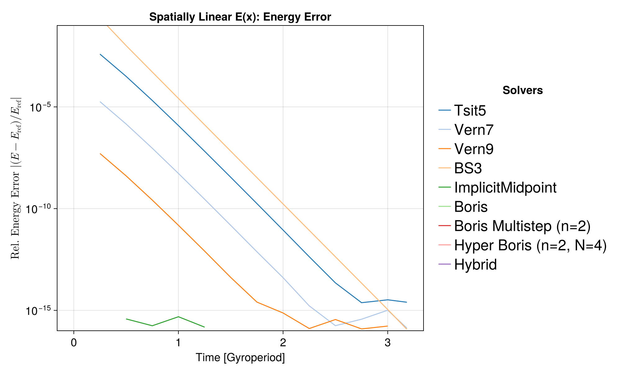
Solver comparisons:

Solver	Max Rel. Error
Tsit5	3.9e-03
Vern7	1.8e-05
Vern9	5.1e-08
BS3	2.3e-01
ImplicitMidpoint	4.9e-16
Boris	6.2e-01
Boris Multistep (n=2)	6.2e-01
Hyper Boris (n=2, N=4)	6.2e-01
Hybrid	9.9e+00

Similar to Case 2a, the Boris solvers systematically show a large error in this case, because of the initial half-step offset.

Case 3: Magnetic Mirror

Energy should be conserved (E=0). The particle bounces back and forth between regions of high magnetic field. We set a divergence-free B field in cylindrical symmetry

$$\begin{array}{rl}{B}_x& =-\alpha B_{0}xz\\ B_y& =-\alpha B_{0}yz\\ B_z& =B_0(1+\alpha z^2)\end{array}$$

function mirror_B(x)
    α = 0.1
    Bz = B₀ * (1 + α * x[3]^2)
    Bx = -B₀ * α * x[1] * x[3]
    By = -B₀ * α * x[2] * x[3]
    return SA[Bx, By, Bz]
end

param3 = prepare(ZeroField(), mirror_B; q = q, m = m)
x0_3 = [0.1, 0.0, 0.0]
v0_3 = [0.5, 0.5, 1.0]
tspan3 = (0.0, 200.0)
E_init_3 = 0.5 * m * norm(v0_3)^2
E_func3(t, x, v) = E_init_3

f, results = run_test(
    "Magnetic Mirror", param3, x0_3, v0_3, tspan3, E_func3;
    dt = T / 20, ymin = 1.0e-16, ymax = 2.0, gc = true, hybrid = true
)

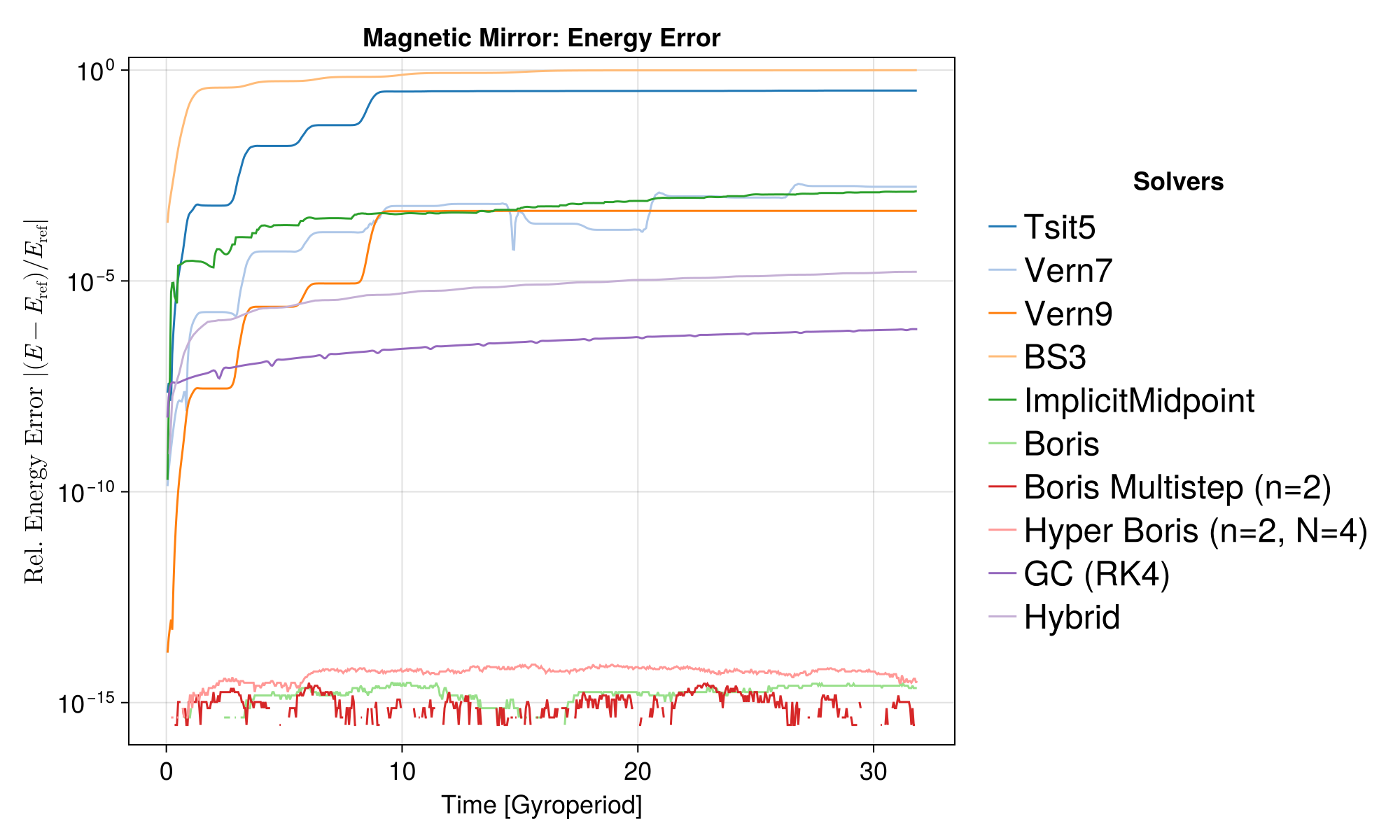
Solver comparisons:

Solver	Max Rel. Error
Tsit5	3.3e-01
Vern7	2.0e-03
Vern9	4.6e-04
BS3	9.9e-01
ImplicitMidpoint	1.3e-03
Boris	3.0e-15
Boris Multistep (n=2)	3.0e-15
Hyper Boris (n=2, N=4)	8.0e-15
GC (RK4)	7.2e-07
Hybrid	1.6e-05

In this magnetic mirror case, a fixed time step larger than 0.05*T leads to numerical instability for many general ODE solvers.

Case 4: E cross B Drift

We test a more complex case from Section 6 of Zenitani & Kato (2025), where both magnetic and electric fields are non-zero. Here we have a constant magnetic field $B_z=B_0$ and a constant electric field with components $E_y=0.5$ and $E_z=0.1$. The particle starts at the origin with zero initial velocity. The analytical kinetic energy gain can be exactly determined from the velocity:

$$\begin{array}{rl}{v}_x(t)& =\frac{E_y}{B_0}[1-\cos (\mathrm{\Omega }t)]\\ v_y(t)& =\frac{E_y}{B_0}\sin (\mathrm{\Omega }t)\\ v_z(t)& =\left(\frac{q{E}_z}{m}\right)t\end{array}$$

const E_y = 0.5
const E_z = 0.1

B_func4(x) = SA[0.0, 0.0, B₀]
E_func4(x, t) = SA[0.0, E_y, E_z]

param4 = prepare(E_func4, B_func4; q, m)
x0_4 = [0.0, 0.0, 0.0]
v0_4 = [0.0, 0.0, 0.0]
tspan4 = (0.0, 200 * T)

function E_ref4(t, x, v)
    Ey2B₀ = E_y / B₀
    vx_theo = Ey2B₀ * (1 - cos(Ω * t))
    vy_theo = Ey2B₀ * sin(Ω * t)
    vz_theo = (q * E_z / m) * t
    return 0.5 * m * (vx_theo^2 + vy_theo^2 + vz_theo^2)
end

f, results = run_test(
    "ExB Drift", param4, x0_4, v0_4, tspan4, E_ref4;
    dt = T / 4, ymin = 1.0e-8, ymax = 1.0e-1, gc = true, hybrid = true,
    gc_phi = x -> -(E_y * x[2] + E_z * x[3]),
    odes = [
        ("Tsit5", Tsit5()),
        ("Vern7", Vern7()),
    ],
    symplectics = []
)

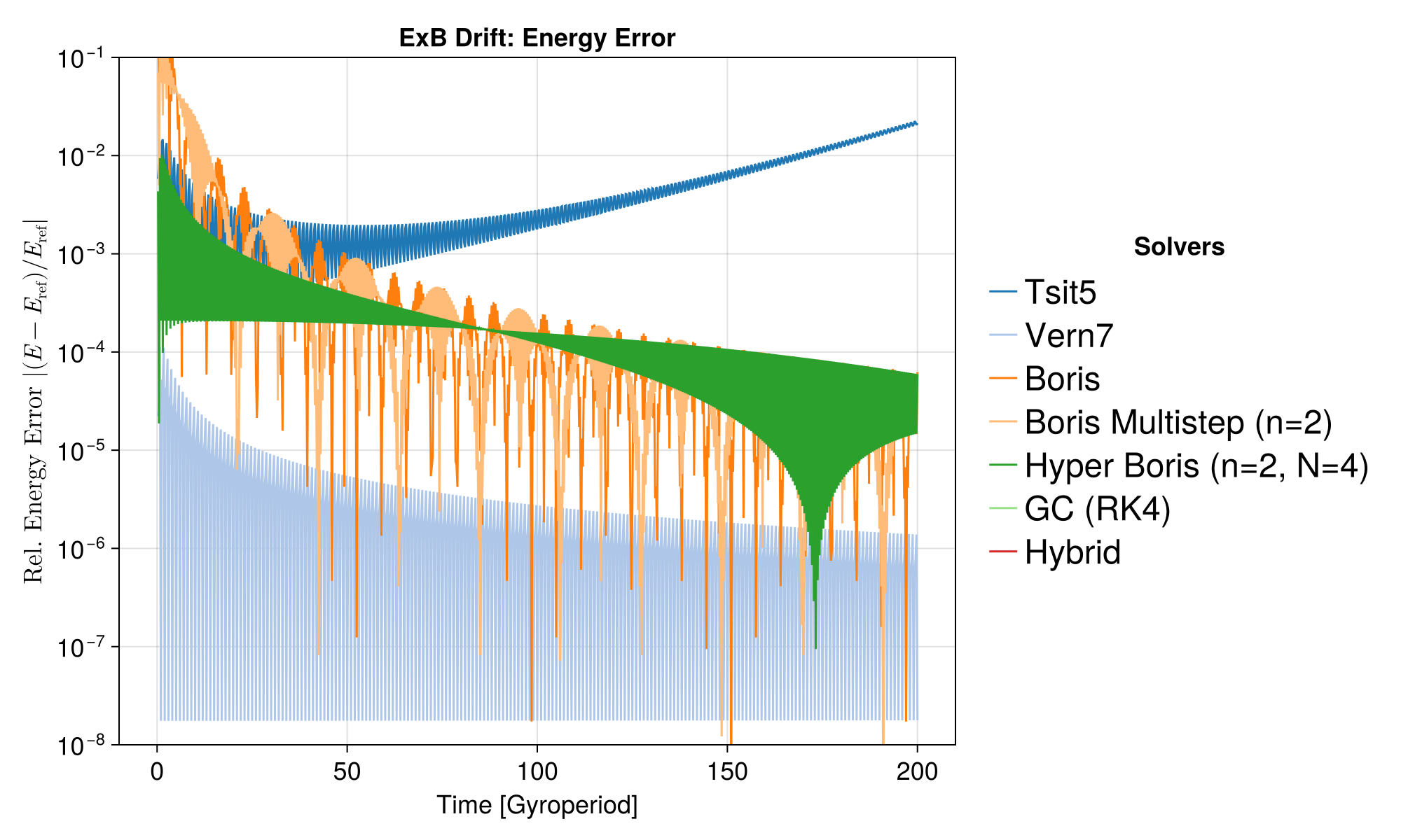
Solver comparisons:

Solver	Max Rel. Error
Tsit5	2.2e-02
Vern7	1.1e-04
Boris	5.4e-01
Boris Multistep (n=2)	1.6e-01
Hyper Boris (n=2, N=4)	1.0e-02
GC (RK4)	1.8e-09
Hybrid	2.0e-16

The relative energy error depends on the order of the solver, while the trend shows the quasi-symplectic property. For Tsit5, the error accumulates over long time and large time steps.