Number Density Calculation

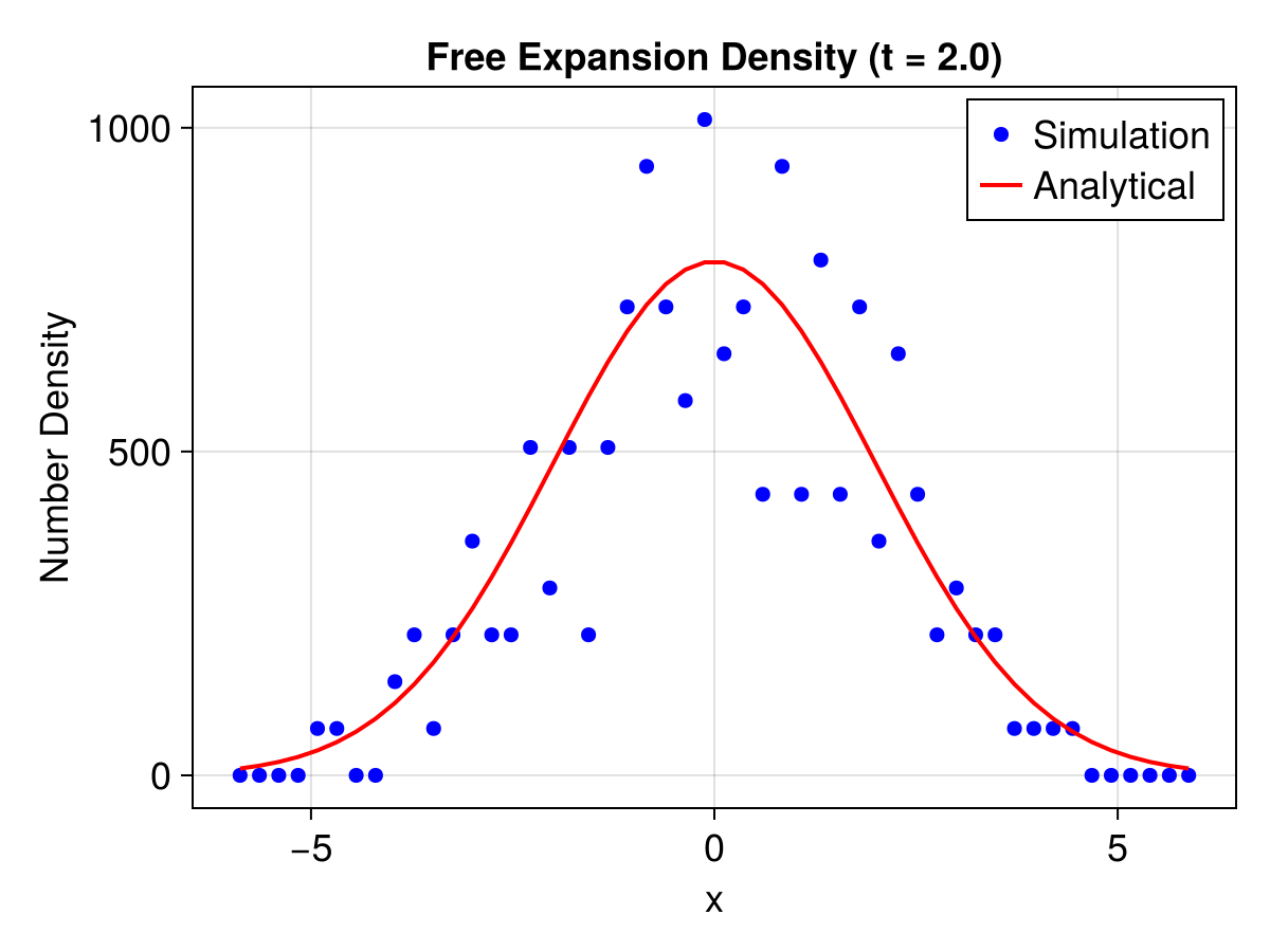
This example demonstrates how to calculate the number density of a group of particles and compares it with the analytical solution for a freely expanding Maxwellian cloud.

using TestParticle
using Meshes
using OrdinaryDiffEq
using StaticArrays
using Statistics
using LinearAlgebra
using Random
using CairoMakie

Random.seed!(1234);

Simulation Setup

Parameters

N = 100_000
m = 1.0
q = 1.0
T = 1.0

1.0

Thermal velocity: $v_{th}=\sqrt{2k_{B}T/m}$

vth = sqrt(2 * T / m)
t_end = 2.0

2.0

Initialize particles Point source at origin: ${\mathbf{r}}_0=\mathbf{0}$

x0 = [SVector(0.0, 0.0, 0.0) for _ in 1:N];

Maxwellian velocity distribution $u_0=0$, $p=n{k}_{B}T=1$ (assuming $n=1$ effectively for distribution shape)

vdf = TestParticle.Maxwellian([0.0, 0.0, 0.0], T, 1.0; m = m)

VelocityDistributionFunctions.ShiftedPDF{Float64, VelocityDistributionFunctions.MaxwellianPDF{Float64}, Vector{Float64}}(
base: VelocityDistributionFunctions.MaxwellianPDF{Float64}(vth=1.4142135623730951)
u0: [0.0, 0.0, 0.0]
)

Use the vectorized rand to get a Vector of SVectors

v0 = rand(vdf, N);

Create TraceProblem template Construct an EnsembleProblem to simulate multiple trajectories.

prob_func(prob, i, repeat) = remake(prob, u0 = vcat(x0[i], v0[i]))

prob_func (generic function with 1 method)

Define a single problem template

u0_dummy = vcat(x0[1], v0[1])
# Zero fields
param = prepare(TestParticle.ZeroField(), TestParticle.ZeroField(); q, m)
tspan = (0.0, t_end)
prob = ODEProblem(trace, u0_dummy, tspan, param);

ensemble_prob = EnsembleProblem(prob; prob_func)

EnsembleProblem with problem ODEProblem

Solve

sols = solve(ensemble_prob, Tsit5(), EnsembleThreads(), trajectories = N);

Density Calculation

Define a grid for density calculation The cloud expands to $r\sim v_{th}{t}_{end}$. With $v_{th}=\sqrt{2}\approx 1.414$ and $t_{end}=2.0$, we have $r\approx 2.8$. We cover $[-6,6]$ to capture the tails.

L = 6.0
dims = (50, 50, 50)
grid = CartesianGrid((-L, -L, -L), (L, L, L); dims)

50×50×50 CartesianGrid
├─ minimum: Point(x: -6.0 m, y: -6.0 m, z: -6.0 m)
├─ maximum: Point(x: 6.0 m, y: 6.0 m, z: 6.0 m)
└─ spacing: (0.24 m, 0.24 m, 0.24 m)

Calculate density at $t_{end}$ get_number_density returns count / volume

density = TestParticle.get_number_density(sols, grid, t_end);

Extract a 1D slice along x-axis (approx. $y=0,z=0$)

mid_y = dims[2] ÷ 2
mid_z = dims[3] ÷ 2
density_x = density[:, mid_y, mid_z];

Grid coordinates for plotting get_cell_centers returns ranges for each dimension

grid_x, grid_y, grid_z = TestParticle.get_cell_centers(grid)
xs_plot = collect(grid_x);

Analytical Solution

The analytical number density $n(\mathbf{r},t)$ for a collisionless gas of $N$ particles expanding from a point source with a Maxwellian velocity distribution $f(\mathbf{v})$ is derived as follows.

The velocity distribution is:

$$f(\mathbf{v})=\frac{1}{(\pi v_{th}^2{)}^{3/2}}\exp (-\frac{v^2}{v_{th}^2})$$

For free expansion, the position of a particle at time $t$ is given by $\mathbf{r}=\mathbf{v}t$. Using the transformation of variables $\mathbf{v}=\mathbf{r}/t$, the volume element transforms as $d^3\mathbf{v}=t^{-3}{d}^3\mathbf{r}$.

Conservation of particle number implies $n(\mathbf{r},t)d^3\mathbf{r}=Nf(\mathbf{v})d^3\mathbf{v}$. Thus:

$$n(\mathbf{r},t)=\frac{N}{t^3}f\left(\frac{\mathbf{r}}{t}\right)=\frac{N}{(\sqrt{\pi }{v}_{th}t{)}^3}\exp (-\frac{r^2}{(v_{th}t{)}^2})$$

Compare with $n(x,0,0,t)$.

r2 = xs_plot .^ 2
sigma_param = vth * t_end
n_analytic = @. N / (sqrt(π) * sigma_param)^3 * exp(-r2 / sigma_param^2);

Visualization

f = Figure(fontsize = 18)
ax = Axis(f[1, 1],
   title = "Free Expansion Density (t = $(t_end))",
   xlabel = "x",
   ylabel = "Number Density")

scatter!(ax, xs_plot, density_x, label = "Simulation", color = :blue, markersize = 10)
lines!(ax, xs_plot, n_analytic, label = "Analytical", color = :red, linewidth = 2)
axislegend(ax)