
Phase Space Tracking
This example validates the three phase-space tracing methods of TestParticle.jl against an analytically known steady-state distribution function (VDF). Unlike the Shock Phase Space demo where the three methods are only compared with each other, here we know the exact VDF at the detector and can quantify how far each reconstruction deviates from it.
Scenario: E×B drift of a bi-Maxwellian
We use a uniform magnetic field
This gives us a rigorous control experiment: any discrepancy between a reconstructed phase-space plot and this analytic expectation is purely numerical (integration error, Monte-Carlo scatter, binning / grid resolution).
using TestParticle
import TestParticle as TP
using LinearAlgebra: norm
using StaticArrays
using Random
using Statistics: mean, var
using VelocityDistributionFunctions
using CairoMakie
using Meshes

seed = 42;
Field and plasma parameters
const B_mag = 10.0e-9  # uniform magnetic field magnitude [T]
const B_vec = SA[0.0, 0.0, B_mag]  # along +z
const V_drift = -400.0e3  # desired E×B drift speed [m/s] (along -x)
# E×B drift: u_E = E×B/B²  ⇒  E = B × u_E  (with E·B = 0).
const E_vec = SA[0.0, B_mag * V_drift, 0.0]  # [V/m]

function get_E_steady(r, t = 0.0)
    return E_vec
end

function get_B_steady(r, t = 0.0)
    return B_vec
end;
Source VDF: drifting bi-Maxwellian
The test distribution is anisotropic (
const n0 = 3.0e6        # number density [m⁻³]
const T_par_eV = 15.0   # parallel temperature [eV]
const T_perp_eV = 45.0  # perpendicular temperature [eV]
const p_par = n0 * TP.qᵢ * T_par_eV
const p_perp = n0 * TP.qᵢ * T_perp_eV

const vdf = TP.BiMaxwellian(
    SA[0.0, 0.0, 1.0], SA[V_drift, 0.0, 0.0], p_par, p_perp, n0; m = TP.mᵢ
);
Geometry and integration
const x_source = SA[300.0e3, 0.0, 0.0] # source plane [m]
const tspan = (0.0, 4.0) # [s]; > transport time 500 km / 400 km/s = 1.25 s
const dt = get_gyroperiod(B_mag) / 40 # [s]

const x_downstream = -200.0e3 # detector plane downstream of the origin [m]

detector_down = Meshes.Plane(
    Meshes.Point(x_downstream, 0.0, 0.0), Meshes.Vec(1.0, 0.0, 0.0)
)

param = prepare(get_E_steady, get_B_steady; species = Proton);
Analytic reference and error metric
The exact detector VDF is the source bi-Maxwellian evaluated at the detector velocity. All three methods reconstruct the 2-D projections
analytic_projectionintegrates over an arbitrary grid, which is used for the 1-D slice and for the grid-based backward method;project_vdfapplied to the analyticfsampled on the bin centers reproduces the binning of the two forward methods, so those are compared bin for bin.
All reconstructions are then scored with the same relative L2 norm
const vlim = 1000.0
const z_int = range(-vlim, vlim; step = 10.0)    # km/s, integration axis
# Source phase-space density [s³/m⁶].
f_src(v) = n0 * pdf(vdf, v)

const v_edges = -1000:20:1000
const centers = bin_centers(v_edges)
const ana_f3d = [
    f_src(SA[vx, vy, vz] * 1.0e3) * 1.0e18 for vx in centers, vy in centers, vz in centers
]

f_xy_ana, f_xz_ana, f_yz_ana = project_vdf(ana_f3d, 20.0)
const ana_hists = (
    (centers, centers, f_xy_ana),
    (centers, centers, f_xz_ana),
    (centers, centers, f_yz_ana),
);
Method 1: Forward Monte Carlo
nparticles matches the trajectory budget of the two other methods, so that the three errors in the deviation report below are directly comparable.
nparticles = 50000

function prob_func_maxwellian(prob, ctx)
    v = rand(ctx.rng, vdf)
    u0 = SA[x_source..., v...]
    return remake(prob, u0 = u0)
end

u0_dummy = SA[0.0, 0.0, 0.0, 0.0, 0.0, 0.0]
prob = TraceProblem(u0_dummy, tspan, param; prob_func = prob_func_maxwellian)

# Warm up the machinery shared by all three methods (ensemble solve, `prob_func`, crossing
# detection), otherwise the compilation cost lands on whichever method happens to run first
# and the per-trajectory costs below are not comparable.
solve(prob, Boris(), EnsembleThreads(); dt, trajectories = 100, seed)

t_mc = @elapsed sols = solve(
    prob, Boris(), EnsembleThreads(); dt,
    trajectories = nparticles, seed
);

function reconstruct_mc_projections(sols, detector, n0, dv_km)
    vxi = [s.u[1][4] for s in sols.u]
    vs, ws_init = get_particle_crossings(sols, detector, vxi)

    v_edges = -1000:dv_km:1000
    centers = bin_centers(v_edges)
    # Each macro-particle stands for $n_0/N$ of the source density spread over one bin
    # volume $dv^3$; the $|v_{x,\mathrm{src}}|/|v_{x,\mathrm{det}}|$ rescale carried by
    # `bin_velocity_space` turns the density-weighted launch ensemble into the crossing
    # flux recorded at the detector and back into a density.
    w = fill(n0 * 1.0e9 / (length(sols.u) * dv_km^3), length(vs))
    f_3d = bin_velocity_space(vs, w, v_edges; vx_source = ws_init)

    f_xy, f_xz, f_yz = project_vdf(f_3d, dv_km)
    return ((centers, centers, f_xy), (centers, centers, f_xz), (centers, centers, f_yz))
end

hists_down = reconstruct_mc_projections(sols, detector_down, n0, 20.0);
Method 2: Forward Liouville Tracking
By Liouville's theorem average = true) estimates the bin-averaged average = false histogram estimator) is the more faithful rendering of the mapped velocity volume, but at dv = 20 km/s the 3 vth sampling sphere only places a handful of samples in each bin, so the counting noise dominates and we average here.
function reconstruct_liouville_projections(sols, detector, vdf, n0; dv_km = 20.0)
    ws0 = [n0 * pdf(vdf, s.u[1][SA[4, 5, 6]]) for s in sols.u]
    vs, ws = get_particle_crossings(sols, detector, ws0)

    v_edges = -1000:dv_km:1000
    centers = bin_centers(v_edges)
    f_3d = bin_velocity_space(vs, ws .* 1.0e18, v_edges; average = true)

    f_xy, f_xz, f_yz = project_vdf(f_3d, dv_km)
    return ((centers, centers, f_xy), (centers, centers, f_xz), (centers, centers, f_yz))
end

nparticles_m2 = 50000
const vth_perp = sqrt(2 * p_perp / (n0 * TP.mᵢ))
const vradius_m2 = 3 * vth_perp

function prob_func_m2(prob, ctx)
    v = sample_velocity_ball(ctx.rng, vradius_m2; center = SA[V_drift, 0.0, 0.0])
    u0 = SA[x_source..., v...]
    return remake(prob, u0 = u0)
end

prob_m2 = TraceProblem(
    SA[0.0, 0.0, 0.0, 0.0, 0.0, 0.0], tspan, param; prob_func = prob_func_m2
)
t_liou = @elapsed sols_m2 = solve(
    prob_m2, Boris(), EnsembleThreads(); dt,
    trajectories = nparticles_m2, seed
);

hists_down_m2 = reconstruct_liouville_projections(
    sols_m2, detector_down, vdf, n0
);
Method 3: Backward Liouville Tracing
const source_plane = Meshes.Plane(Meshes.Point(x_source...), Meshes.Vec(1.0, 0.0, 0.0))

function reconstruct_backward_projections(
        detector_x, dt, param;
        v_range = 1000.0e3, vy_range = 400.0e3, dv_km = 20.0,
        adaptive = true, dv_coarse_km = 80.0, margin_km = 150.0
    )
    dv = dv_km * 1.0e3
    bounds = ((-v_range, v_range), (-vy_range, vy_range), (-v_range, v_range))

    t_solve = @elapsed begin
        f_3d_km, (vx_grid, vy_grid, vz_grid) = vdf_backward_trace(
            param, detector_x, source_plane, f_src;
            v_range, vy_range, vz_range = v_range, dv, dt, tspan = (0.0, -8.0),
            adaptive, dv_coarse = dv_coarse_km * 1.0e3, margin = margin_km * 1.0e3,
            relthresh = 1.0e-5, bounds,
            isoutside = (u, p, t) -> u[1] < detector_x - 1.0e5 ||
                u[1] > x_source[1] + 100.0e3
        )
    end
    nparticles_bw = length(vx_grid) * length(vy_grid) * length(vz_grid)

    f_xy, f_xz, f_yz = project_vdf(f_3d_km, dv_km)
    # Drop the negligible tail. Zeroing rather than `NaN`-ing keeps those cells at the
    # floor of the log colour scale below (a `NaN` would render transparent, unlike the
    # empty bins of the other three rows) and keeps them out of the log-scaled slice.
    for f in (f_xy, f_xz, f_yz)
        f[f .< maximum(f) * 1.0e-6] .= 0.0
    end

    return (
            (vx_grid .* 1.0e-3, vy_grid .* 1.0e-3, f_xy),
            (vx_grid .* 1.0e-3, vz_grid .* 1.0e-3, f_xz),
            (vy_grid .* 1.0e-3, vz_grid .* 1.0e-3, f_yz),
        ), t_solve, nparticles_bw
end

res_down_bw, t_bw_down, n_bw_down =
    reconstruct_backward_projections(x_downstream, dt, param);
Phase space comparison
The three reconstructions are shown next to the analytic reference for each 2-D velocity projection at the downstream detector.
function plot_validation(h_mc, h_liou, h_bw, h_ana, xloc; vlim = 1000.0, rel = 1.0e-5)
    titles = ["Analytic", "Monte Carlo", "Forward Liouville", "Backward Liouville"]
    hists = (h_ana, h_mc, h_liou, h_bw)
    nrows = 4
    xlab = [L"V_x [\mathrm{km/s}]", L"V_x [\mathrm{km/s}]", L"V_y [\mathrm{km/s}]"]
    ylab = [L"V_y [\mathrm{km/s}]", L"V_z [\mathrm{km/s}]", L"V_z [\mathrm{km/s}]"]
    fig = Figure(size = (1400, 1500), fontsize = 28)
    gl = fig[1, 1] = GridLayout()
    Label(
        gl[1, 2:4],
        "Detector at x = $(round(xloc * 1.0e-3; digits = 0)) km";
        fontsize = 32, tellwidth = false
    )
    global_max = maximum(
        maximum(filter(isfinite, vec(hists[r][i][3]))) for r in 1:nrows, i in 1:3
    )
    cr = (rel * global_max, global_max)
    last_hm = nothing
    for r in 1:nrows, i in 1:3
        ax = Axis(
            gl[r + 1, i + 1], xlabel = xlab[i], ylabel = ylab[i];
            xlabelsize = 28, ylabelsize = 28, titlesize = 24,
            xticklabelsize = 22, yticklabelsize = 22,
            limits = (-vlim, vlim, -vlim, vlim), aspect = 1
        )
        last_hm = heatmap!(
            ax, hists[r][i]...;
            colormap = :turbo, colorscale = Makie.pseudolog10, colorrange = cr
        )
    end
    Colorbar(
        fig[1, 2], last_hm;
        label = L"f\ [\mathrm{s}^2/\mathrm{km}^5]", labelsize = 24, ticklabelsize = 18
    )
    for r in 1:nrows
        Label(gl[r + 1, 1], titles[r]; fontsize = 22, rotation = π / 2, tellheight = false)
    end
    return fig
end

fig_down = plot_validation(hists_down, hists_down_m2, res_down_bw, ana_hists, x_downstream)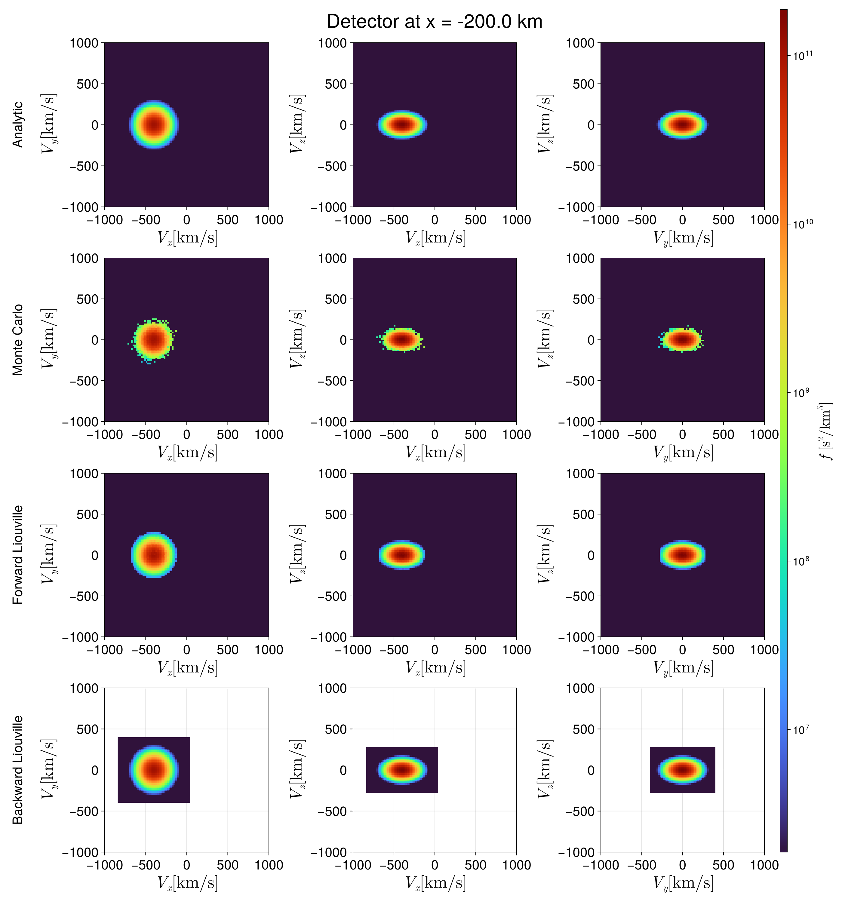
1-D slice check
Slice the
function slice_at(h, second::Bool, val)
    g1, g2, M = h
    if second
        return g1, M[:, argmin(abs.(g2 .- val))]
    else
        return g2, M[argmin(abs.(g1 .- val)), :]
    end
end

const fine_x = range(-vlim, vlim; step = 10.0)
const fana_slice = [
    analytic_projection(f_src, 2, [vx], [0.0], z_int, step(z_int))[1] for vx in fine_x
]

xc_f, fy_f = slice_at(hists_down[2], true, 0.0)
xc_l, fy_l = slice_at(hists_down_m2[2], true, 0.0)
xc_b, fy_b = slice_at(res_down_bw[2], true, 0.0)

# Log-scaled slice: stretching the low-density wings makes the Monte-Carlo scatter
# (where the methods deviate most from the analytic profile) directly visible.
function _logslice(xc, fy)
    m = fy .> 0
    return xc[m], fy[m]
end
xc_f_l, fy_f_l = _logslice(xc_f, fy_f)
xc_l_l, fy_l_l = _logslice(xc_l, fy_l)
xc_b_l, fy_b_l = _logslice(xc_b, fy_b)

fig_slice = Figure(size = (900, 500), fontsize = 24)
axs = Axis(
    fig_slice[1, 1], xlabel = L"V_x [\mathrm{km/s}]",
    ylabel = L"\log_{10} f(V_x, V_z=0)",
    yscale = log10, limits = (-vlim, 0.0, 1.0e7, 1.0e12)
)
# Bang Wong's colour-blind-safe palette. Green and red are skipped on purpose: they are the
# pair that deuteranopia and protanopia collapse onto each other.
const wc = Makie.wong_colors()
lines!(axs, fine_x, fana_slice; label = "Analytic", color = :black, linewidth = 3, linestyle = :dash)
scatterlines!(
    axs, xc_f_l, fy_f_l; label = "Monte Carlo", color = wc[1],
    linewidth = 2, markersize = 13
)
scatterlines!(
    axs, xc_l_l, fy_l_l; label = "Forward Liouville", color = wc[6],
    linewidth = 2, markersize = 13
)
lines!(axs, xc_b_l, fy_b_l; label = "Backward Liouville", color = wc[4], linewidth = 2.5)
axislegend(axs; position = :lt, framevisible = false)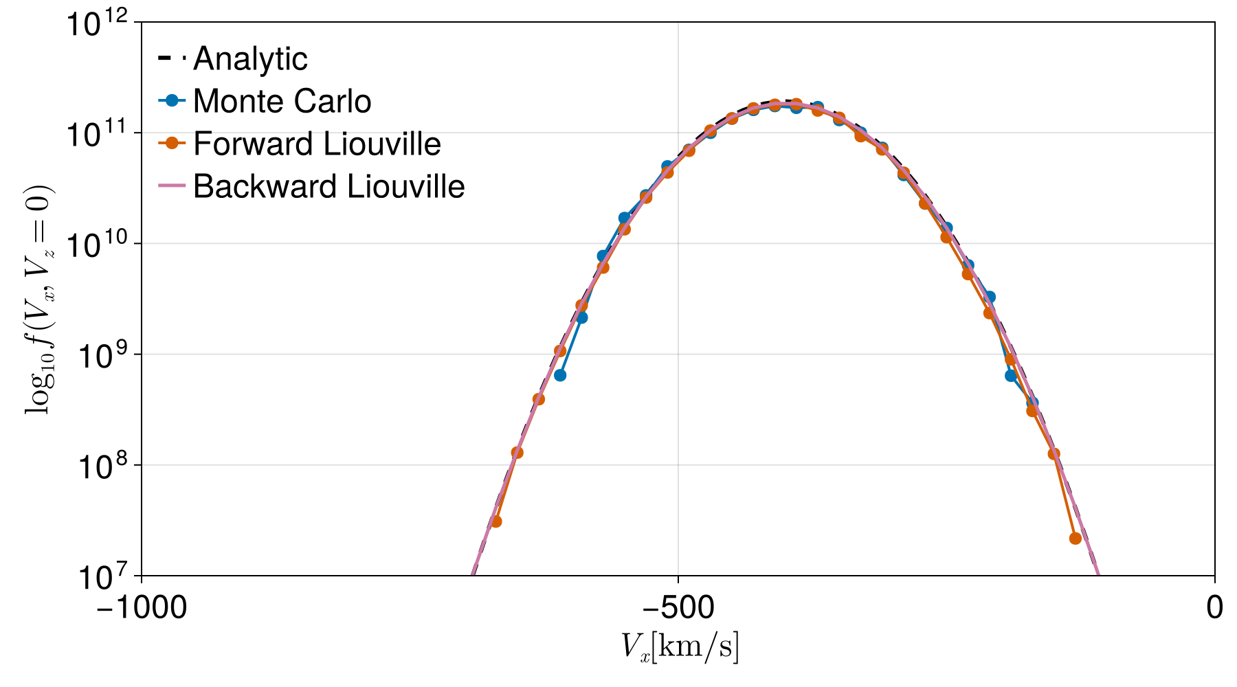
Deviation report
One number per method: the three 2-D projections are pooled and the relative L2 norm is taken over the union, so the number does not depend on how the density happens to project onto each velocity plane.
All three methods are given the same budget of ≈5·10⁴ trajectories, so both the errors and the costs are directly comparable. The two forward methods are statistical, with error ∝ 1/√N; the backward method has no statistical noise and its error is set by the grid resolution instead, which is why it wins on accuracy while spending about twice as much per trajectory.
mats(h::Tuple) = (h[1][3], h[2][3], h[3][3])
pooled_relative_l2(recs, refs) = relative_l2(
    reduce(vcat, (vec(A) for A in recs)), reduce(vcat, (vec(A) for A in refs))
)

t_per_mc = t_mc / nparticles * 1.0e6
t_per_liou = t_liou / nparticles_m2 * 1.0e6
t_per_bw = t_bw_down / n_bw_down * 1.0e6| Method | Rel. L2 error | Trajectories | Time [s] | Cost [µs/traj] |
|---|---|---|---|---|
| Monte Carlo | 0.0473 | 50000 | 1.42 | 28.4 |
| Forward Liouville | 0.0597 | 50000 | 1.40 | 28.0 |
| Backward Liouville | 0.0034 | 49280 | 2.18 | 44.2 |
What the results tell us
Backward Liouville is the most accurate (0.34% error, exact up to grid resolution). Because it traces directly backward from the target detector grid to the source, there is zero statistical noise and uniform coverage across the distribution, including the tails. It is also the most expensive per trajectory, since a backward trajectory has to run until it reaches the source plane, with every step stored.
Monte Carlo is limited by statistical noise (
). With the trajectories used here, its relative deviation is ~4.7%, matching theoretical Poisson noise. Reaching the 0.34% of Backward Liouville would need ~200× more trajectories, of order 10⁷, which at the per-trajectory costs above is ~100× the compute. Forward Liouville provides smooth bin-averaged phase-space densities, but exhibits an outer boundary artifact caused by truncating the source velocity sampling to a finite sphere (
). In addition, forward trajectories that miss the detector or fall outside the populated region do not contribute to the target.
Monte-Carlo sampling noise scales as 1/√N
The report above quotes Monte Carlo at ≈5% and attributes it to N, repeating each N with many independent seed realizations, and measure the sampling noise as the relative RMS scatter of the reconstructed histogram across realizations. For a multinomial (Monte-Carlo) estimator the per-bin density has standard deviation
vec_of(h) = vcat([vec(p[3]) for p in h]...)

function run_mc_N(N, rseed)
    function prob_func(prob, ctx)
        v = rand(ctx.rng, vdf)
        u0 = SA[x_source..., v...]
        return remake(prob, u0 = u0)
    end
    u0_dummy = SA[0.0, 0.0, 0.0, 0.0, 0.0, 0.0]
    prob = TraceProblem(u0_dummy, tspan, param; prob_func = prob_func)
    sols = solve(
        prob, Boris(), EnsembleThreads(); dt,
        trajectories = N, seed = rseed
    )
    return reconstruct_mc_projections(sols, detector_down, n0, 20.0)
end

const Ns = [1000, 2000, 4000, 8000]
const nseeds = 24

agg_noise = Float64[]   # relative RMS scatter of the histogram across seeds → ∝ 1/√N
agg_var = Float64[]   # total histogram variance across seeds → ∝ 1/N
ana_l2 = Float64[]   # analytic relative L2 per seed (averaged over projections)

for N in Ns
    hs = [run_mc_N(N, s) for s in 1:nseeds]
    vecs = [vec_of(h) for h in hs]

    l2s = [mean(relative_l2(h[i][3], ana_hists[i][3]) for i in 1:3) for h in hs]
    push!(ana_l2, mean(l2s))

    mean_vec = mean(vecs)
    mask = mean_vec .> maximum(mean_vec) * 1.0e-4
    mv = mean_vec[mask]
    res = [norm(v[mask] .- mv) / norm(mv) for v in vecs]
    push!(agg_noise, mean(res))

    mat = reduce(hcat, [v[mask] for v in vecs])   # bins × seeds
    push!(agg_var, sum(var(mat; dims = 2)))
end

function logslope(x, y)
    lx = log10.(Float64.(x)); ly = log10.(y)
    return sum((lx .- mean(lx)) .* (ly .- mean(ly))) / sum((lx .- mean(lx)) .^ 2)
end
slope_noise = logslope(Ns, agg_noise)   # target ≈ -0.5
slope_var = logslope(Ns, agg_var)     # target ≈ -1.0

fig_scaling = Figure(size = (700, 460), fontsize = 24)
ax1 = Axis(
    fig_scaling[1, 1], xscale = log10, yscale = log10,
    xlabel = L"N\ \mathrm{[trajectories]}",
    ylabel = L"MC\ noise\ (rel.\ RMS\ scatter)",
    title = "Sampling noise ∝ 1/√N  (slope = $(round(slope_noise; digits = 2)))"
)
scatter!(ax1, Float64.(Ns), agg_noise; color = :blue, markersize = 8, label = "measured")
ref1 = agg_noise[end] * sqrt(Ns[end]) ./ sqrt.(Float64.(Ns))
lines!(ax1, Float64.(Ns), ref1; color = :black, linestyle = :dash, label = L"\propto 1/\sqrt{N}")
axislegend(ax1; position = :rt)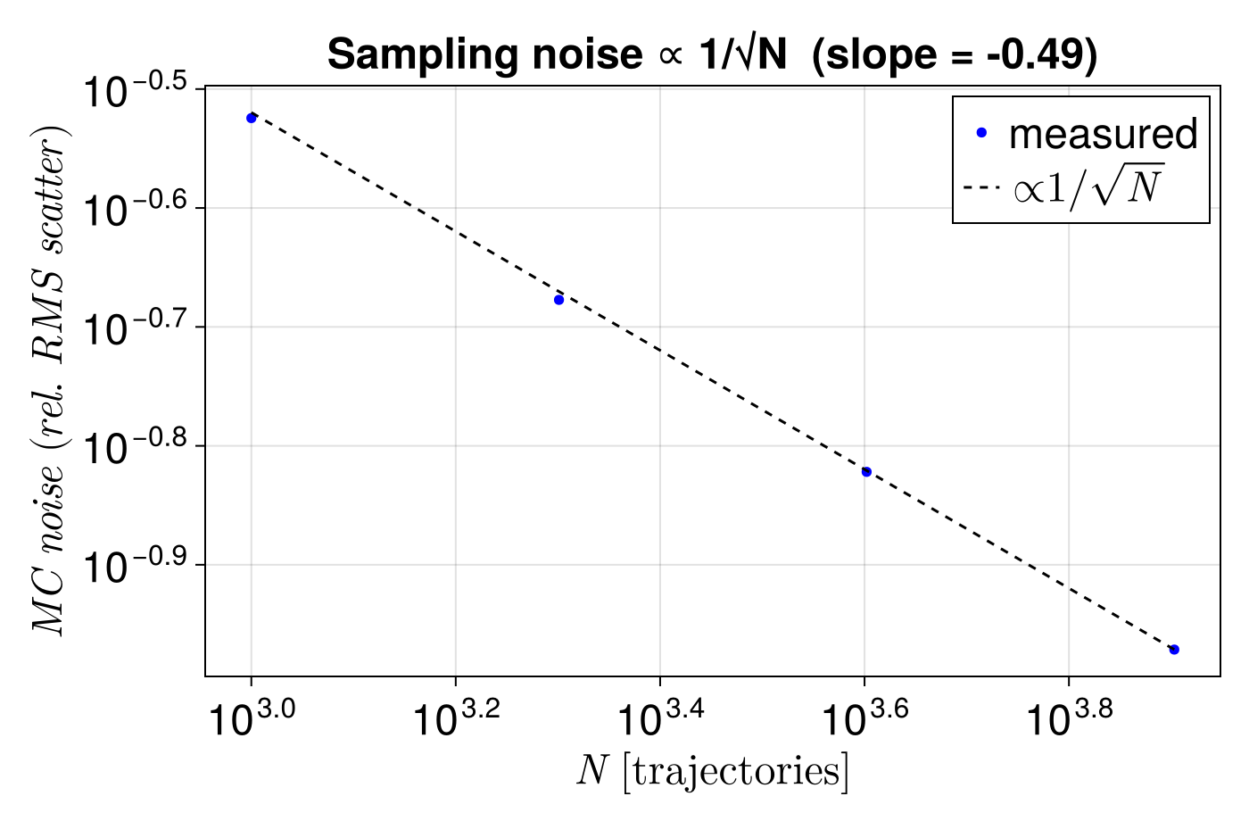
The measured log–log slope is close to −0.5, confirming the expected 1/√N sampling-noise scaling: the ≈5% Monte-Carlo deviation above is dominated by Monte-Carlo scatter, not by method bias.
| N (trajectories) | MC noise (∝ 1/√N) | ΣVar (∝ 1/N) | analytic L2 |
|---|---|---|---|
| 1000 | 0.2989 | 1.72e+23 | 0.3107 |
| 2000 | 0.2102 | 8.51e+22 | 0.2185 |
| 4000 | 0.1507 | 4.35e+22 | 0.1567 |
| 8000 | 0.1068 | 2.18e+22 | 0.1116 |