Magnetic Drift and Energy Partition

This example demonstrates the combined magnetic drift (curvature + grad-B) of a single charged particle and how it partitions between the parallel and perpendicular kinetic energies. It is the direct numerical test of the question raised in issue #61: in a field where curvature and grad-B are coupled, are the two drifts a single "magnetic drift" distinguished only by the energy partition?

More theoretical details can be found in Magnetic Drift and Fundamentals of Plasma Physics by Paul Bellan, §3.6.

using TestParticle, OrdinaryDiffEq, StaticArrays
using LinearAlgebra: norm, ×, ⋅, normalize
using ForwardDiff: jacobian
using CairoMakie

Field and drift deduction

We use a 2D azimuthal field that circles the z-axis with radius r: B = B₀ (x₂, -x₁, 0) / r². It has both a curved field line (curvature radius R_c = r) and a perpendicular magnitude gradient (|B| = B₀/r), and the two are coupled through B·R_c = B₀ = const. With E = 0 the guiding-center velocity (mirroring trace_gc_drifts!) is

$${\mathbf{v}}_{\mathrm{gc}}=\frac{m}{2q{B}^2}(\mathbf{b}\times \mathrm{\nabla }B)v_{\perp }^2+\frac{m}{qB}(\mathbf{b}\times \mathit{\kappa })v_{\parallel }^2,\mathit{\kappa }=(\mathbf{b}\cdot \mathrm{\nabla })\mathbf{b}.$$

For this field both (b×∇B) and (b×κ) point along -ẑ and their denominators collapse to the same constant B₀, giving the clean combined form

$$v_z=-\frac{m}{q{B}_0}(v_{\parallel }^2+\frac{v_{\perp }^2}{2}).$$

So curvature drift carries the v_\parallel^2 part and grad-B drift carries the v_\perp^2/2 part of one and the same magnetic drift.

const Bmag0 = 1.0e-7

curve_B(x) = SA[x[2] / norm(x[1:2])^2, -x[1] / norm(x[1:2])^2, 0.0] * Bmag0
zero_E(x) = SA[0.0, 0.0, 0.0];

Analytic guiding-center drift evaluated directly from the field function, using exactly the same quantities (∇B from the B-Jacobian, κ from JB·b) as the package's get_B_parameters / trace_gc_drifts!. This is the "code tracing" reference against which we compare the Boris-traced orbit.

function analytic_drift(x, v, q, m)
    B = curve_B(x)
    Bmag = norm(B)
    b = B / Bmag
    JB = jacobian(curve_B, x)
    ∇B = JB' * b
    κ = (JB * b + b * (-(∇B ⋅ b))) / Bmag
    Ω = (q / m) * Bmag
    vpar = v ⋅ b
    vperp = v - vpar * b
    wsq = vperp ⋅ vperp
    return wsq * (b × ∇B) / (2Ω * Bmag) + vpar^2 * (b × κ) / Ω
end;

Pitch-angle scan

We launch protons from the same point x0 with a fixed speed v0 but varying pitch angle α between v and b, i.e. v_\parallel = v0 cos α, v_\perp = v0 sin α. The predicted drift is then compared to the drift of the guiding center obtained from the full Boris orbit.

x0 = SA[1.0, 0.0, 0.0]
b0 = normalize(curve_B(x0))   # b = (0, -1, 0) at x0
eperp = SA[0.0, 0.0, 1.0]     # perpendicular to b at x0
const v0 = 1.0
tspan = (0.0, 30.0)
n = 9
αs = range(0, π / 2; length = n)

q, m = Proton.q, Proton.m

param = prepare(zero_E, curve_B, species = Proton)
gc = get_gc_func(param)

function scan_magnetic_drift(αs, v0, x0, b0, eperp, q, m, param, gc, tspan)
    n = length(αs)
    vpar_list = Vector{Float64}(undef, n)
    vperp_list = Vector{Float64}(undef, n)
    theory_z = Vector{Float64}(undef, n)
    meas_z = Vector{Float64}(undef, n)

    ts = range(tspan..., length = 400)
    A = hcat(ones(length(ts)), ts)

    # Sample a trace to fix the element type of the solutions vector.
    stateinit0 = [x0..., (v0 * b0)...]
    prob0 = ODEProblem(trace!, stateinit0, tspan, param)
    sol0 = solve(prob0, Vern9(); abstol = 1.0e-10, reltol = 1.0e-10)
    sols = Vector{typeof(sol0)}(undef, n)

    for (i, α) in enumerate(αs)
        vpar = v0 * cos(α)
        vperp = v0 * sin(α)
        v = vpar * b0 + vperp * eperp
        vpar_list[i] = vpar
        vperp_list[i] = vperp

        # Theoretical prediction from the field itself.
        theory_z[i] = analytic_drift(x0, v, q, m)[3]

        # Boris trace.
        stateinit = [x0..., v...]
        prob = ODEProblem(trace!, stateinit, tspan, param)
        sol = solve(prob, Vern9(); abstol = 1.0e-10, reltol = 1.0e-10)
        sols[i] = sol

        # Drift of the guiding center: slope of its z position vs time.
        z_gc = [gc(sol(t))[3] for t in ts]
        meas_z[i] = (A \ z_gc)[2]
    end

    return vpar_list, vperp_list, theory_z, meas_z, sols
end

vpar_list, vperp_list, theory_z, meas_z, sols =
    scan_magnetic_drift(αs, v0, x0, b0, eperp, q, m, param, gc, tspan)

([1.0, 0.9807852804032304, 0.9238795325112867, 0.8314696123025452, 0.7071067811865476, 0.5555702330196023, 0.38268343236508984, 0.19509032201612833, 6.123233995736766e-17], [0.0, 0.19509032201612825, 0.3826834323650898, 0.5555702330196022, 0.7071067811865475, 0.8314696123025452, 0.9238795325112867, 0.9807852804032304, 1.0], [-0.10439684914853153, -0.10241016490814782, -0.09675256685325757, -0.08828537300146379, -0.07829763686139865, -0.06830990072133353, -0.05984270686953973, -0.054185108814649496, -0.05219842457426577], [-0.10274930770562365, -0.09899449338234752, -0.09229331014085823, -0.08368505663076214, -0.07437809448869219, -0.0655878293308667, -0.058423535720998857, -0.05374815011773663, -0.05212737422875149], SciMLBase.ODESolution{Float64, 2, Vector{Vector{Float64}}, Nothing, Nothing, Vector{Float64}, Vector{Vector{Vector{Float64}}}, Nothing, SciMLBase.ODEProblem{Vector{Float64}, Tuple{Float64, Float64}, true, Tuple{Float64, Float64, TestParticle.Field{false, typeof(Main.zero_E)}, TestParticle.Field{false, typeof(Main.curve_B)}, ZeroField}, SciMLBase.ODEFunction{true, SciMLBase.AutoSpecialize, FunctionWrappersWrappers.FunctionWrappersWrapper{Tuple{FunctionWrappers.FunctionWrapper{Nothing, Tuple{Vector{Float64}, Vector{Float64}, Tuple{Float64, Float64, TestParticle.Field{false, typeof(Main.zero_E)}, TestParticle.Field{false, typeof(Main.curve_B)}, ZeroField}, Float64}}}, FunctionWrappersWrappers.AllowNonIsBits, FunctionWrappersWrappers.SingleCacheStorage}, LinearAlgebra.UniformScaling{Bool}, Nothing, Nothing, Nothing, Nothing, Nothing, Nothing, Nothing, Nothing, Nothing, Nothing, Nothing, Nothing, typeof(SciMLBase.DEFAULT_OBSERVED), Nothing, Nothing, Nothing, Nothing}, Base.Pairs{Symbol, Union{}, Nothing, @NamedTuple{}}, SciMLBase.StandardODEProblem}, OrdinaryDiffEqVerner.Vern9{typeof(OrdinaryDiffEqCore.trivial_limiter!), typeof(OrdinaryDiffEqCore.trivial_limiter!), FastBroadcast.Serial, Val{true}}, OrdinaryDiffEqCore.InterpolationData{SciMLBase.ODEFunction{true, SciMLBase.AutoSpecialize, FunctionWrappersWrappers.FunctionWrappersWrapper{Tuple{FunctionWrappers.FunctionWrapper{Nothing, Tuple{Vector{Float64}, Vector{Float64}, Tuple{Float64, Float64, TestParticle.Field{false, typeof(Main.zero_E)}, TestParticle.Field{false, typeof(Main.curve_B)}, ZeroField}, Float64}}}, FunctionWrappersWrappers.AllowNonIsBits, FunctionWrappersWrappers.SingleCacheStorage}, LinearAlgebra.UniformScaling{Bool}, Nothing, Nothing, Nothing, Nothing, Nothing, Nothing, Nothing, Nothing, Nothing, Nothing, Nothing, Nothing, typeof(SciMLBase.DEFAULT_OBSERVED), Nothing, Nothing, Nothing, Nothing}, Vector{Vector{Float64}}, Vector{Float64}, Vector{Vector{Vector{Float64}}}, Nothing, OrdinaryDiffEqVerner.Vern9Cache{Vector{Float64}, Vector{Float64}, Vector{Float64}, typeof(OrdinaryDiffEqCore.trivial_limiter!), typeof(OrdinaryDiffEqCore.trivial_limiter!), FastBroadcast.Serial, Val{true}}, Nothing}, SciMLBase.DEStats, Nothing, Nothing, Nothing, Nothing}[[1.0 0.9999903761527952 … -0.49060104629101825 -0.46806175321137516; 0.0 -0.039889855682987724 … 0.888219049584545 0.8975385777482492; … ; -1.0 -0.9999712401799022 … 0.39242379058999677 0.3661405233322393; 0.0 -0.0075228264674451935 … -0.1398135962510569 -0.11666165552703242], [1.0 1.0012079846149042 … -0.8476407219990083 -0.8530587994665373; 0.0 -0.03555647927186079 … -0.5806781973648071 -0.5632157556626589; … ; -0.9807852804032304 -0.9819324011900963 … 0.9519304960277812 0.9557361263554013; 0.19509032201612825 0.17748954734161054 … -0.06443364099595472 -0.015364182064997406], [1.0 1.0022130482233833 … 1.0100783966808613 1.0071674857550141; 0.0 -0.03232121823500736 … -0.011786686247273685 -0.021191799344006283; … ; -0.9238795325112867 -0.925873289346124 … -0.9112009636322891 -0.9116826135755344; 0.3826834323650898 0.356529777712086 … 0.2859752703335916 0.3121522422008156], [1.0 1.003098172043117 … -1.005247698097061 -1.0148606579736121; 0.0 -0.028554975076625043 … -0.08423984268729182 -0.0664671865933466; … ; -0.8314696123025452 -0.8339873591757345 … 0.7952297297361873 0.7883332600809096; 0.5555702330196022 0.5220596689584612 … 0.47191892728160284 0.3937697627774853], [1.0 1.0038603730007463 … 0.8494808365970792 0.8759958230153316; 0.0 -0.024026007938831657 … 0.764143101729782 0.758491534280319; … ; -0.7071067811865476 -0.709777508730193 … -0.0985027342247938 -0.2237360453083713; 0.7071067811865475 0.6674574250371768 … -0.5698039081574015 -0.7041723720529448], [1.0 1.0044817485075104 … 0.23486337143212735 0.2214713670338084; 0.0 -0.018757456222198824 … -1.0332860085093336 -1.020725699058517; … ; -0.5555702330196023 -0.5580077001238634 … 0.6691328712192205 0.6087603724562718; 0.8314696123025452 0.7869657812385185 … 0.27655878656019833 0.4146418054998759], [1.0 1.0049428529796485 … -1.202633069930923 -1.2066242828099494; 0.0 -0.012872841541372256 … 0.019973956379629676 0.023297222422616275; … ; -0.38268343236508984 -0.3845356708262869 … 0.32525908416260224 0.3239997128102438; 0.9238795325112867 0.8758635964405338 … -0.8448642744996898 -0.8770653577969788], [1.0 1.0052272514532619 … 0.053674285562507175 0.060614457790290864; 0.0 -0.006550201763488175 … 1.040407701338477 1.0657933231863959; … ; -0.19509032201612833 -0.19608905961646145 … 0.7757347021352168 0.9049888073645622; 0.9807852804032304 0.9306413686613801 … 0.5886121809319288 0.3549611838584873], [1.0 1.005323588739191 … 1.0146689938192643 1.019798734688847; 0.0 -2.054746591021134e-18 … -1.5128346856445174e-15 -1.5210491562178394e-15; … ; -6.123233995736766e-17 -6.155160123481194e-17 … -8.198971566420178e-16 -9.30155788411759e-16; 1.0 0.9491414867858052 … 0.8605087705128437 0.8122042087202367]])

Validation

Scatter of the Boris-traced guiding-center drift against the analytic drift computed directly from the field function (should lie on the y = x line), and the linear dependence on the energy partition (v_\parallel^2 + v_\perp^2/2).

fig = Figure(size = (1500, 500), fontsize = 22)

ax3 = Axis3(
    fig[1, 1]; title = "Sample trajectories", xlabel = "x", ylabel = "y",
    zlabel = "z", aspect = :data
)
for idx in (1, 5, 9)   # α = 0 (curvature only), 45° (mixed), 90° (grad-B only)
    lines!(
        ax3, sols[idx]; idxs = (1, 2, 3),
        label = "α = $(round(rad2deg(αs[idx]); digits = 0))°"
    )
end
axislegend(ax3, framevisible = true, backgroundcolor = (:white, 0.6))

ax_conf = Axis(
    fig[1, 2]; title = "Code tracing confirmation",
    xlabel = "Analytic drift vz [m/s]", ylabel = "Measured drift vz [m/s]",
    aspect = 1
)
scatter!(ax_conf, theory_z, meas_z; markersize = 10)
xr = extrema(theory_z)
lines!(
    ax_conf, [xr[1], xr[2]], [xr[1], xr[2]]; color = :red, linestyle = :dash,
    label = "y = x"
)
axislegend(ax_conf, position = :lt)

ax_part = Axis(
    fig[1, 3]; title = "Energy partition",
    xlabel = "v∥² + v⊥²/2  [m²/s²]", ylabel = "Drift vz [m/s]"
)
X = vpar_list .^ 2 .+ 0.5 .* (vperp_list .^ 2)
scatter!(ax_part, X, meas_z; markersize = 10, color = :black, label = "measured")
slope = (X' * X) \ (X' * meas_z)   # least-squares slope
xs = range(extrema(X)...; length = 50)
lines!(ax_part, xs, slope[1] .* xs; color = :blue, label = "linear fit")
axislegend(ax_part, position = :lt)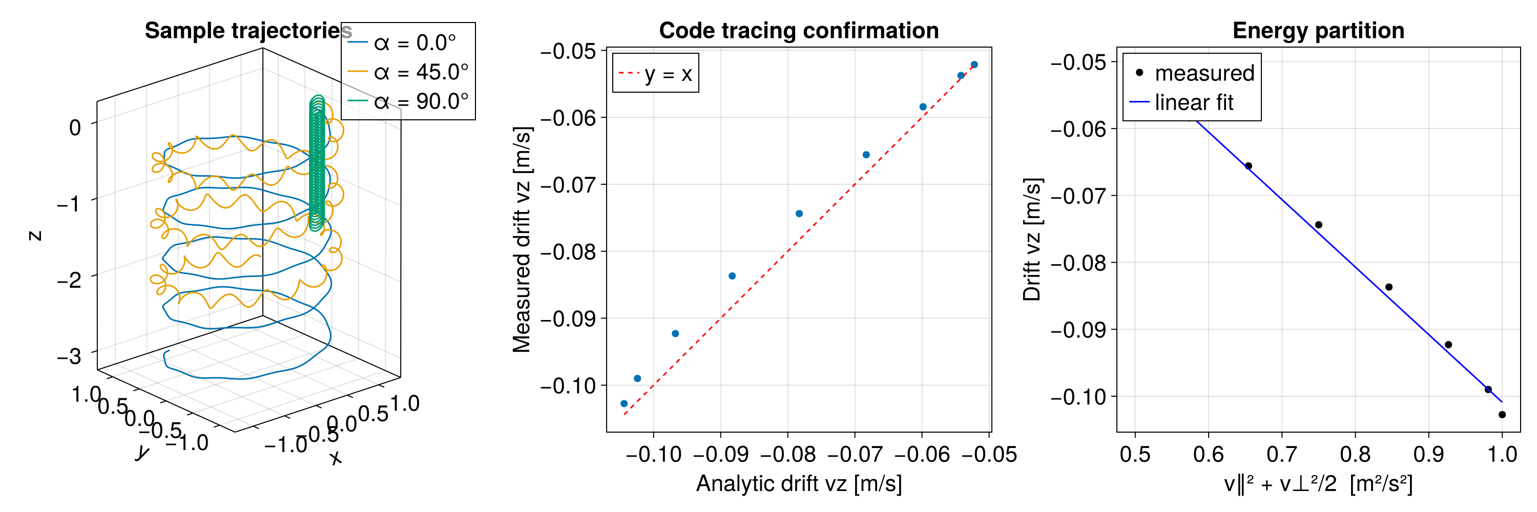

The fitted slope equals m/(q B₀) to within the (small) finite-Larmor-radius correction; the grad-B and curvature parts therefore carry the v⊥²/2 and v∥² weights, i.e. they are one magnetic drift, not two independent forces.