TestParticle.jl
Test-particle tracing in analytical or numerical fields (via Meshes.jl and FastInterpolations.jl) using SciML ODE solvers and native particle pushers. For theoretical background, see Single-Particle Motions.
Installation
using Pkg
Pkg.add("TestParticle")
Load a solver package (OrdinaryDiffEqVerner / OrdinaryDiffEq or BorisPushers) for integration, and GLMakie / CairoMakie / Plots when plotting trajectories.
Usage
Trace a proton in a 10 nT uniform magnetic field (SI units by default) using TraceProblem with either a SciML ODE solver or native BorisPushers.jl:
julia> using TestParticle, OrdinaryDiffEqVerner, BorisPushers, StaticArrays

julia> B(x) = SA[0.0, 0.0, 1.0e-8];

julia> u0 = [1.0, 0.0, 0.0, 0.0, 1.0, 0.1];

julia> tspan = (0.0, 20.0);

julia> param = prepare(; B, species = Proton);

julia> prob = TraceProblem(u0, tspan, param);

julia> sol = solve(prob, Vern7());

julia> dt = 1.0e-2;

julia> sol_boris = solve(prob, Boris(); dt, saveat = 10 * dt);

julia> sol_hyper = solve(prob, MultistepBoris6(; n = 4); dt);

julia> sol_adapt = solve(prob, AdaptiveBoris(; safety = 0.1));

julia> all(s -> s.retcode == TestParticle.ReturnCode.Success, (sol, sol_boris, sol_hyper, sol_adapt))
true
Pass a Vector u0 for in-place RHS evaluation or an SVector for out-of-place evaluation.
Models and Solvers
| Model | Setup & Problem | State u0 | Solvers | Guide |
|---|---|---|---|---|
FullOrbit (default) | p = prepare(; E, B, F)<br>TraceProblem(u0, tspan, p) | [x..., v...] | Boris, MultistepBoris6, AdaptiveBoris, SciML ODE | Boris Pusher |
RelativisticOrbit | p = prepare(; E, B, F)<br>TraceProblem{RelativisticOrbit}(u0, tspan, p) | [x..., γv...] | SciML ODE (Vern7, Vern9, ...) | Numerical Methods |
GuidingCenter | u0_gc, p_gc = prepare_gc(u0; E, B)<br>TraceGCProblem(u0_gc, tspan, p_gc) | [X..., v∥] | SciML ODE (Vern7, RK4, ...) | Guiding Center |
| Hybrid GC–FO | p = prepare(; E, B)<br>TraceProblem(u0, tspan, p) | [x..., v...] | AdaptiveHybrid(; dtmax) | Hybrid GC-FO Solver |
Canonical / RelativisticCanonical | p = prepare_canonical(; phi, A)<br>TraceCanonicalProblem(u0, tspan, p) | [x..., p...] | SciML ODE / symplectic | Canonical Tracing Form |
Numerical grids: interpolate array fields with
build_interpolatorbeforeprepare.Ensembles & GPUs: pass
EnsembleThreads(),EnsembleDistributed(), or aKernelAbstractionsGPU backend tosolve.Examples: browse worked cases under Examples or the sidebar sections.
Performance and Scaling
Tracing many particles can be computationally intensive. TestParticle.jl is designed to scale across multiple cores and machines using Julia's built-in parallel computing capabilities.
Serial Performance
The following table compares the performance of TestParticle's Boris solver against standard ODE solvers from DifferentialEquations.jl for a single particle simulation. Reproducible benchmark scripts are available in benchmark/bench_serial.jl.
Benchmark Configuration:
Hardware: Intel Core Ultra 7 265K (20 cores, 20 threads)
Task: Simulating 1 particle for 0.1 second with
steps, saving endpoint).
| Solver | Median Time | Speedup | Allocations | Memory |
|---|---|---|---|---|
| TestParticle Boris | 477 ms | 1.0x | 91 | 4.83 KiB |
| ODE Tsit5 (fixed) | 10392 ms | 22x slower | 66 | 4.04 KiB |
| ODE Vern9 (fixed) | 24962 ms | 52x slower | 74 | 4.70 KiB |
Parallel Scaling
TestParticle.jl supports multithreading, distributed computing, and multi-node parallelism for ensemble simulations on CPUs. The following aggregate throughput was obtained on Perlmutter CPU nodes (2x AMD EPYC 7763, 128 physical cores per node). Each ensemble traces 16384 particles for 250000 Boris steps in a uniform magnetic field, saving 100 points per trajectory. Every point is the median of repeated runs, and the error bars span the fastest and slowest repetition.
Multithreading:
EnsembleThreads()over 1 to 128 threads in one process.Distributed:
EnsembleDistributed()over 1 to 128 worker processes on one node.Multi-node:
EnsembleSplitThreads()with one worker per node, each worker running 128 threads, over 1 to 8 nodes.
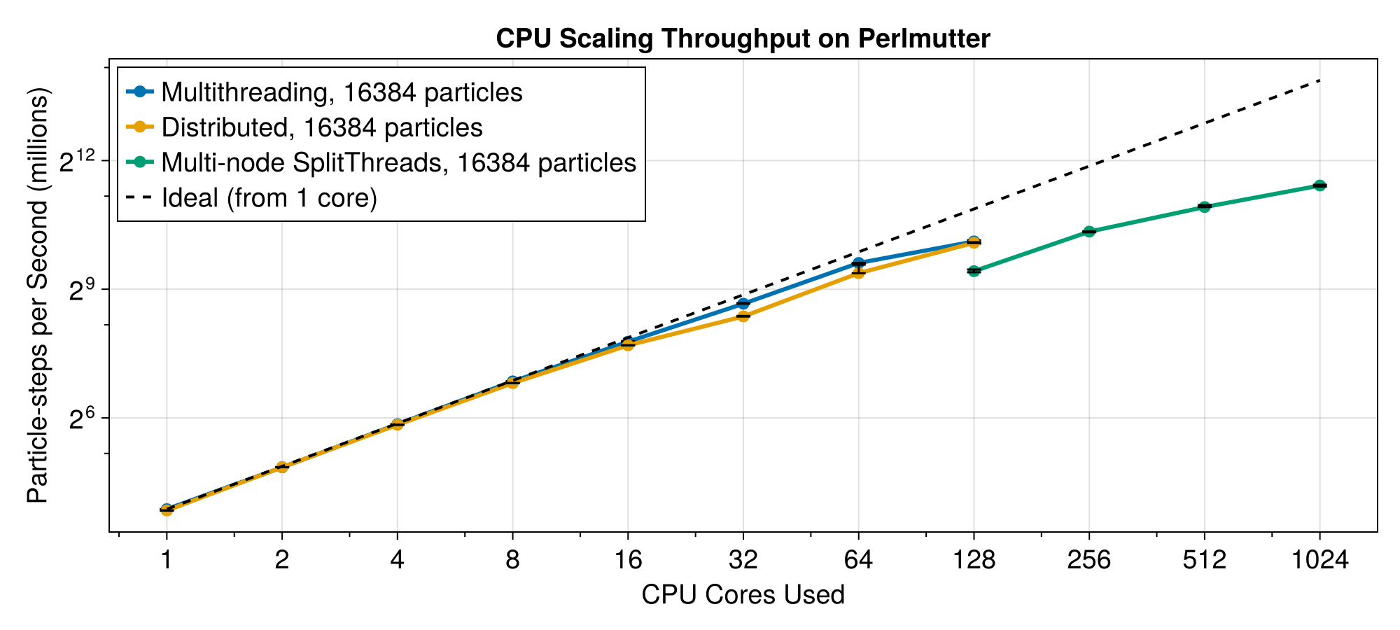
The two single-node strategies track each other within a few percent and reach about 1.1 billion particle-steps per second on 128 cores, close to 60 percent of the single-core rate extrapolated linearly; the rest goes to the lower clock an all-core load draws. Multi-node carries on past one node and reaches 2.7 billion particle-steps per second across 8 nodes, but its one-node point sits well below the single-process runs, since EnsembleSplitThreads gathers every trajectory back to the master process, a cost the shared-memory path does not pay.
Reproducible scripts and the recorded measurements live in benchmark; render the figure with benchmark/plot_scaling.jl cpu.
GPU Performance and Multi-Backend Scaling
TestParticle.jl provides vendor-agnostic GPU acceleration via KernelAbstractions.jl. Passing a GPU backend such as CUDA.CUDABackend(), AMDGPU.ROCBackend(), Metal.MetalBackend(), or oneAPI.oneAPIBackend() to solve(prob, Boris(), backend) executes the Boris pusher kernels directly on hardware accelerators.
Benchmark Environments:
Workstation (Consumer GPU): Intel Core Ultra 7 265K (20 cores, 20 threads), NVIDIA GeForce RTX 5070 (12 GB GDDR7)
HPC Node (Datacenter GPU): NERSC Perlmutter node, AMD EPYC 7763 (128 threads), NVIDIA A100-SXM4-40GB
Reproducible benchmark scripts are available in benchmark/compare_boris_backends.jl.
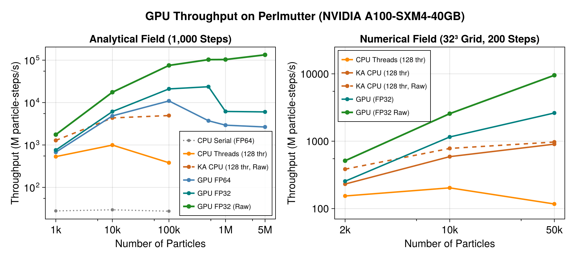
The aggregate throughput scaling across ensemble sizes on Perlmutter (NVIDIA A100-SXM4-40GB and 128-thread AMD EPYC 7763) is shown below, contrasting an analytical field with a numerical 3D discrete grid field:
Render the figure with benchmark/plot_scaling.jl gpu.
Key observations from the scaling throughput:
CPU Multithreading Contention (
CPU Threadsthroughput drops from ~1,000 M steps/s atODESolutionwrapper objects across 128 threads creates heavy heap allocation contention and garbage collection (GC) pressure. By contrast,KA CPUbatches particle states and maintains ~4,100 M steps/s.GPU Default API Bottleneck (
ODESolutionJulia objects.Unlocking Full Hardware Throughput with Raw Output: Switching to
raw_output = trueand a bulk initial state matrix (u0) eliminates all per-particle host object allocations. Particle states remain in contiguous matrix buffers, allowing GPU FP32 throughput to scale continuously to over
1. Analytical Field Tracing (1,000 steps)
Times below report the median wall time for an ensemble of particles traced over 1,000 steps on the RTX 5070 workstation. Speeds in parentheses are relative to CPU Serial:
| Number of Particles | CPU Serial (FP64) | CPU Threads (20 Thr) | KA CPU (FP64) | GPU (FP64) | GPU (FP32) |
|---|---|---|---|---|---|
| 1,000 | 14.15 ms | 1.62 ms (8.7x) | 0.79 ms (18.0x) | 2.27 ms (6.2x) | 0.52 ms (27.4x) |
| 10,000 | 167.31 ms | 12.89 ms (13.0x) | 5.76 ms (29.1x) | 3.09 ms (54.2x) | 0.85 ms (196.9x) |
| 100,000 | 1521.67 ms | 166.30 ms (9.2x) | 43.22 ms (35.2x) | 23.40 ms (65.0x) | 5.30 ms (286.9x) |
When returning raw matrix output (raw_output = true with a bulk initial state matrix, omitting per-particle ODESolution wrapper assembly), host overhead is eliminated: at
2. Numerical Grid Field Interpolation (
For discrete electromagnetic grids, TestParticle.jl automatically converts grid interpolations into device-native GPUGrid structures with hardware register trilinear evaluation:
| Number of Particles | CPU Threads (20 Thr) | KA CPU (Fair Baseline) | GPU (Default API) | GPU (Raw Output) |
|---|---|---|---|---|
| 2,000 | 3.39 ms | 1.67 ms (2.0x) | 0.95 ms (3.6x) | 0.75 ms (4.5x) |
| 10,000 | 11.29 ms | 6.34 ms (1.8x) | 1.64 ms (6.9x) | 0.74 ms (15.3x) |
| 50,000 | 79.71 ms | 23.99 ms (3.3x) | 4.40 ms (18.1x) | 1.26 ms (63.3x) |
`CPU Threads` allocates one `ODESolution` per particle, which dominates the runtime for grid fields. `KA CPU` provides the fair parallel CPU baseline by batching particle updates without per-particle object allocation overhead.
3. Kernel Isolation and Theoretical Peak Performance
Because Boris integration holds particle coordinates and velocities entirely in GPU registers throughout the step loop, the kernel performs zero DRAM reads or writes between
Comparing the measured kernel compute against theoretical peak hardware limits reveals the architectural trade-offs between datacenter and consumer GPUs:
| Accelerator | Precision | Kernel Throughput | Measured Compute | Peak Hardware Vector Compute | % of Peak Compute |
|---|---|---|---|---|---|
| NVIDIA A100<br>(Datacenter) | FP32 | 385.1 G steps/s | 20.0 TFLOPS | 19.5 TFLOPS | ~100% |
| FP64 | 191.6 G steps/s | 10.0 TFLOPS | 9.7 TFLOPS | ~100% | |
| NVIDIA RTX 5070<br>(Consumer) | FP32 | 625.4 G steps/s | 31.2 TFLOPS | 38.8 TFLOPS | >80% |
| FP64 | 9.4 G steps/s | 0.49 TFLOPS | 0.61 TFLOPS | ~80% |
Datacenter GPU (A100): Hardware ALUs are engineered with a full-rate 2:1 FP32:FP64 ratio. The Boris pusher achieves ~100% of the peak theoretical vector compute in both precisions, yielding an exact 2.00x speedup for FP32 over FP64.
Consumer GPU (RTX 5070): Consumer GeForce architectures feature a 1:64 hardware ALU rate for FP64. While FP32 delivers exceptional compute (31.2 TFLOPS, >80% of peak), FP64 suffers a 62.4x slowdown due to this hardware throttle.
Numerical Grid Interpolation: Evaluating discrete grids (
grid) transitions the bottleneck from pure ALU compute to GPU L1/L2 cache read bandwidth during trilinear interpolations, sustaining 55.5 G steps/s on the A100 and 48.2 G steps/s on the RTX 5070.
Precision Considerations: Float64 vs Float32
TestParticle.jl supports both double precision (Float64) and single precision (Float32) tracing. Supplying Float32 coordinates, velocities, or time span automatically promotes the simulation parameters, physical constants, and equations to single precision.
Advantages of Float32
Consumer GPU Throughput: Consumer-grade GPUs (e.g., NVIDIA GeForce RTX 30/40/50 series) feature a 1:64 FP64 ALU throughput throttle. Where single precision is physically acceptable, switching to
Float32unlocks the full hardware compute rate, yielding over 60x faster pure kernel execution. On datacenter GPUs (e.g., NVIDIA A100),Float32yields the theoretical 2x speedup over full-rate FP64 ALUs.Lower Memory Footprint: Halves VRAM and host memory consumption for trajectory buffers and 3D electromagnetic grids, reducing memory bandwidth pressure.
Reduced Host Overhead: Memory allocations and data transfers across the PCIe bus are halved in size.
Trade-offs and Limitations of Float32
Accumulated Numerical Drift: With 24 bits of mantissa (~7 significant decimal digits), rounding errors accumulate over long integration periods (
gyro-orbits), potentially leading to phase errors or slight artificial energy drift in non-integrable fields. Dynamic Range / Catastrophic Cancellation: In unnormalized SI units with large coordinate baselines (e.g. planetary magnetospheres where
Float32suffers from catastrophic cancellation in spatial increments.
Computing Resource and Scaling Guidelines
Based on our CPU and GPU scaling benchmarks across problem sizes, architectures, and precisions:
| Problem Scale | Recommended Backend & Configuration | Rationale |
|---|---|---|
| Small Ensembles( | CPU Serial or EnsembleThreads() | Low particle counts cannot saturate GPUs; GPU initialization and kernel launch latency dominate runtime. |
| Medium Ensembles( | EnsembleThreads(), KA.CPU(), or GPU (default API) | Both multi-threaded CPU and GPU scale efficiently. Standard ODESolution wrapper objects allow full SciML ecosystem integration without noticeable allocation bottlenecks. |
| Large Ensembles( | GPU Backend with raw_output = true and bulk u0 matrix | Avoid default per-particle ODESolution wrappers. Allocating |
Precision Guidelines (Accuracy First):
Prioritize Numerical Accuracy: Never sacrifice necessary physical precision for execution speed. Use
Float64by default for single-particle orbits, long integrations (gyro-orbits), and planetary-scale coordinate baselines ( When to Use
Float32: Single precision should only be used when physical error tolerances allow, such as large statistical ensembles using normalized dimensionless units (e.g., coordinates scaled by gyroradius or ion inertial length).Hardware Implications:
When
Float64is required, datacenter GPUs (A100/H100) or CPU clusters are the ideal targets, as datacenter GPUs maintain full-rate FP64 ALUs (incurring only an expected ~2x compute difference relative to FP32).Consumer GPUs (GeForce RTX series) throttle FP64 ALUs to a 1:64 rate. While they execute
Float64with full mathematical correctness, hardware throughput is restricted. When FP64 is needed, choose datacenter GPUs or multi-core CPUs rather than downgrading precision toFloat32.
Electromagnetic Field Grids: Construct numerical fields with
build_interpolator, then pass them toprepare(; E, B). Supported interpolators are converted to device grids by the GPU solver; see the constructor documentation for boundary and order restrictions.
Presentations
For interactive presentations and educational materials, please check out these Pluto notebooks:
Publications
Zijin Zhang, Anton V. Artemyev, and Vassilis Angelopoulos, 2025, "Quantification of ion scattering by solar-wind current sheets: Pitch-angle diffusion rates", Phys. Rev. E, https://doi.org/10.1103/pkzv-k5t3
Chi Zhang, Hongyang Zhou, Chuanfei Dong, Yuki Harada, Masatoshi Yamauchi, Shaosui Xu, Hans Nilsson, et al. 2024. “Source of Drift-Dispersed Electrons in Martian Crustal Magnetic Fields”, The Astrophysical Journal, https://doi.org/10.3847/1538-4357/ad64d5.
Acknowledgement
TestParticle.jl is acknowledged by citing the Zenodo DOI:  .
Nothing can be done such easily without the support of the Julia community. We appreciate all the contributions from developers around the world.