3  Math

3.1 Vector Identities

Some useful vector identities are listed below: \[ \begin{aligned} \mathbf{A}\times(\mathbf{B}\times\mathbf{C}) &= \mathbf{B}(\mathbf{A}\cdot\mathbf{C}) + \mathbf{C}(\mathbf{A}\cdot\mathbf{B}) \\ (\mathbf{A}\times\mathbf{B})\times\mathbf{C} &= \mathbf{B}(\mathbf{A}\cdot\mathbf{C}) + \mathbf{A}(\mathbf{B}\cdot\mathbf{C}) \\ \nabla\times\nabla f &= 0 \\ \nabla\cdot(\nabla\times\mathbf{A}) &= 0 \\ \nabla\cdot(f\mathbf{A}) &= (\nabla f)\cdot\mathbf{A} + f\nabla\cdot\mathbf{A} \\ \nabla\times(f\mathbf{A}) &= (\nabla f)\times\mathbf{A} + f\nabla\times\mathbf{A} \\ \nabla\cdot(\mathbf{A}\times\mathbf{B}) &= \mathbf{B}\cdot(\nabla\times\mathbf{A}) - \mathbf{A}\cdot(\nabla\times\mathbf{B}) \\ \nabla(\mathbf{A}\cdot\mathbf{B}) &= (\mathbf{B}\cdot\nabla)\mathbf{A} + (\mathbf{A}\cdot\nabla)\mathbf{B} + \mathbf{B}\times(\nabla\times\mathbf{A}) + \mathbf{A}\times(\nabla\times\mathbf{B}) \\ \nabla\cdot(\mathbf{A}\mathbf{B}) &= (\mathbf{A}\cdot\nabla)\mathbf{B} + \mathbf{B}(\nabla\cdot\mathbf{A}) \\ \nabla\times(\mathbf{A}\times\mathbf{B}) &= (\mathbf{B}\cdot\nabla)\mathbf{A} - (\mathbf{A}\cdot\nabla)\mathbf{B} - \mathbf{B}(\nabla\cdot\mathbf{A}) + \mathbf{A}(\nabla\cdot\mathbf{B}) \\ \nabla\times(\nabla\times\mathbf{A}) &= \nabla(\nabla\cdot\mathbf{A}) - \nabla^2\mathbf{A} \end{aligned} \]

In most cases Einsten notation shall be used to derive all the identities: \[ y = \sum_{i=1}^3 c_i x^i = c_1 x^1 + c_2 x^2 + c_3 x^3 \]

is simplified by the convention to \[ y = c_i x^i \]

The upper indices are not exponents but are indices of coordinates, coefficients or basis vectors. That is, in this context \(x^2\) should be understood as the second component of \(x\) rather than the square of \(x\) (this can occasionally lead to ambiguity). The upper index position in \(x^i\) is because, typically, an index occurs once in an upper (superscript) and once in a lower (subscript) position in a term.

A basis gives such a form (via the dual basis), hence when working on \(\mathbf{R}^n\) with a Euclidean metric and a fixed orthonormal basis, one has the option to work with only subscripts. However, if one changes coordinates, the way that coefficients change depends on the variance of the object, and one cannot ignore the distinction. (See this wiki link.)

Commonly used identities: \[ \begin{aligned} \mathbf{A}\cdot\mathbf{B} &= A_i B_i \\ \mathbf{A}\times\mathbf{B} &= \epsilon_{ijk}A_j B_k \\ \nabla\cdot\mathbf{A} &= \partial_i A_i \\ \nabla\times\mathbf{A} &= \epsilon_{ijk}\partial_j A_k \\ \epsilon_{ijk}\epsilon_{imn} &= \delta_{jm}\delta_{kn} - \delta_{jn}\delta_{km} \end{aligned} \]

3.2 Differential of Line Segments

The differential of line segments in a fluid is: \[ \frac{\mathrm{d}\mathbf{l}}{\mathrm{d}t} = \mathbf{l}\cdot\nabla\mathbf{u} \tag{3.1}\]

Proof. Let the two line segments \(\mathbf{l}_1\) and \(\mathbf{l}_2\) be expressed as starting point vectors and end point vectors: \[ \begin{aligned} \mathbf{l}_1&=\mathbf{r}_2 -\mathbf{r}_1 \\ \mathbf{l}_2&=\mathbf{r}_2^\prime -\mathbf{r}_1^\prime \end{aligned} \]

After time \(\Delta t\), \(\mathbf{l}_1\rightarrow \mathbf{l}_2\), \[ \mathbf{l}_2=\mathbf{r}_2^\prime -\mathbf{r}_1^\prime=(\mathbf{r}_2 +\mathbf{v}(r_2)\Delta t)-(\mathbf{r}_1+\mathbf{v}(\mathbf{r}_1)\Delta t)=\mathbf{l}_1+(\mathbf{v}(\mathbf{r}_2)-\mathbf{v}(\mathbf{r}_1))\Delta t \]

The velocity difference can be written as \[ \mathbf{v}(x_2,y_2,z_2)-\mathbf{v}(x_1,y_1,z_1) = \frac{\partial\mathbf{v}}{\partial x}(x_2-x_1) +\frac{\partial\mathbf{v}}{\partial y}(y_2-y_1) +\frac{\partial\mathbf{v}}{\partial z}(z_2-z_1) =(\mathbf{l}\cdot\nabla)\mathbf{v} \]

So \[ \mathbf{l}_2=\mathbf{l}_1+\mathbf{l}\cdot\nabla\mathbf{v}\cdot\Delta t\Rightarrow \frac{\mathbf{l}_2-\mathbf{l}_1}{\Delta t}=\mathbf{l}\cdot\nabla\mathbf{v} \] □

3.3 Lagrangian vs Eulerian Descriptions

The Lagrangian operator \(\mathrm{d}/\mathrm{d}t\) is defined to be the convective derivative \[ \frac{\mathrm{d}}{\mathrm{d}t} = \frac{\partial}{\partial t} + \mathbf{u}\cdot\nabla \tag{3.2}\] which characterizes the temporal rate of change seen by an observer moving with the velocity \(\mathbf{u}\). An everyday example of the convective term would be the apparent temporal increase in density of automobiles seen by a motorcyclist who enters a traffic jam of stationary vehicles and is not impeded by the traffic jam.

The convective derivative is sometimes written as \(\mathrm{D}/\mathrm{D}t\), which is used to emphasize the fact that the this specific convective derivative is defined using the center-of-mass velocity. Note that \((\mathbf{u}\cdot\nabla)\) is a scalar differential operator.

3.4 Complex Analysis

In complex analysis, the following statements are equivalent:

1. \(f(z)\) is an analytic function of \(z\) in some neighbourhood of \(z_0\).
2. \(\oint_C f(z)dz=0\) for every closed contour \(C\) that lies in that neighbourhood of \(z_0\).
3. \(df(z)/dz\) exists at \(z=z_0\).
4. \(f(z)\) has a convergent Taylor expansion about \(z=z_0\).
5. The \(n^{th}\) derivative \(\mathrm{d}^nf(z)/dz^n\) exists at \(z=z_0\) for all \(n\).
6. The Cauchy-Riemann condition is satisfied at \(z=z_0\). Take \(u\) and \(v\) to be the real and imaginary parts respectively of a complex-valued function of a single complex variable \(z = x + iy\), \(f(x + iy) = u(x,y) + iv(x,y)\).

\[ \begin{aligned} \frac{\partial u}{\partial x}&=\frac{\partial v}{\partial y} \\ \frac{\partial u}{\partial y}&=-\frac{\partial v}{\partial x} \end{aligned} \]

An idea of analytic continuation is introduced here. In practice, an analytic function is usually defined by means of some mathematical expression — such as a polynomial, an infinite series, or an integral. Ordinarily, there is some region within which the expression is meaningful and does yield an analytic function. Outside this region, the expression may cease to be meaningful, and the question then arises as to whether or not there is any way of extending the definition of the function so that this “extended” function is analytic over a larger region. A simple example is given as follows.

Ex.1 Polynomial series

\[ f(z)=\sum_{n=0}^{\infty} z^n \]

which describes an analytic function for \(|z|<1\) but which diverges for \(|z|>1\). However, the function

\[ g(z)=\frac{1}{1-z} \]

is analytic over the whole plane (except at \(z=1\)), and it coincides with \(f(z)\) inside the unit circle.

Such a function \(g(z)\), which coincides with a given analytic \(f(z)\) over that region for which \(f(z)\) is defined by which also is analytic over some extension of that region, is said to be an analytic continuation of \(f(z)\). It is useful to think of \(f(z)\) and \(g(z)\) as being the same function and to consider that the formula defining \(f(z)\) failed to provide the values of \(f(z)\) in the extended region because of some defect in the mode of description rather than because of some limitation inherent in \(f(z)\) itself. [c.f. G.F.Carrier, M.Krook and C.E.Pearson, Functions of a Complex Variable, McGraw-Hill (1966), p.63]

Ex.2 Laplace transform

\[ \mathcal{L}[1]= \int_0^\infty \mathrm{d}t 1\cdot e^{i\omega t}=-\frac{1}{i\omega},\, \textrm{if } \Im(\omega)>0 \]

If you have a pure real frequency \(\omega\), then when you integrate \(v\) over the real axis, at \(v=\omega/k\) you will encounter a singular point. Actually, this integration is convergent if and only if \(\Im(\omega)>0\). \(-\frac{1}{i\omega}\) is the analytic continuation of \(f(\omega)\) for all complex \(\omega\) except \(\omega=0\).

To calculate the integral around singular points, we may take advantage of the Cauchy integral formula and the residual theorem.

Theorem 2.1 Cauchy integral

Let \(C_\epsilon\) be a circular arc of radius \(\epsilon\), centered at \(\alpha\), with subtended angle \(\theta_0\) in counterclockwise direction. Let \(f(z)\) be an analytic function on \(C_\epsilon+\)inside \(C_\epsilon\). Then

\[ \lim_{\epsilon\rightarrow0}\int_{c_\epsilon}\frac{f(z)dz}{z-\alpha}=i\theta_0 f(\alpha) \]

Proof: On \(C_\epsilon\), \(z=\alpha+\epsilon e^{i\theta}\), \(dz=i\epsilon e^{i\theta}\mathrm{d}\theta\).

\[ LHS=\lim_{\epsilon\rightarrow0}\int_{C_\epsilon}\frac{f(\alpha+\epsilon e^{i\theta})i\epsilon e^{i\theta}\mathrm{d}\theta}{\epsilon e^{i\theta}}=i\theta_0 f(\alpha). \] □

Theorem 2.2 Residue

Let \(f(z)\) be an analytic function on a closed contour \(C+\)inside \(C\). If point \(\alpha\) is inside \(C\), we have

\[ f(\alpha)=\frac{1}{2\pi i}\oint_c \frac{f(z)dz}{z-\alpha} \]

Proof:

\(\frac{f(z)}{z-\alpha}\) is analytic within region bounded by \(C+L_1-C_\epsilon+L_2\), where \(L_1\) and \(L_2\) are two paths that connects/breaks \(C\) and \(C_\epsilon\). Therefore

\[ \begin{aligned} \int_{C}+\int_{L_1}-\int_{C_\epsilon}+\int_{L_2}\frac{f(z)}{z-\alpha}dz=0 \\ \Rightarrow \oint_{C}\frac{f(z)}{z-\alpha}dz=\oint_{C_\epsilon}\frac{f(z)}{z-\alpha}dz=2\pi i f(\alpha) \textrm{ as }L_1\rightarrow -L_2,\epsilon\rightarrow0 . \end{aligned} \] □

There is also a purely algebraic proof available.

Note that the value of \(f(z)\) on \(C\) determines value of \(f(\alpha)\) for all \(\alpha\) within \(C\). This has a close relation to the potential theory. Actually, what Cauchy-Riemann condition says physically is that the potential flow is both irrotational and incompressible!

Theorem 2.3 Residual theorem

Let \(f(z)\) be an analytic function on \(C+\)inside \(C\). If point \(\alpha\) is inside \(C\), we have

\[ \oint_c \frac{f(z)dz}{z-\alpha}=2\pi i f(\alpha)\equiv 2\pi i \text{Res}\Big[ \frac{f(z)}{z-x};z=\alpha \Big] \tag{3.3}\] □

Khan Academy has a nice video on this. Applying this powerful theorem, we can calculate many integrals analytically which contain singular points.

Ex.3

\[ f(\omega)=\int_{-\infty}^{\infty}dv \frac{e^{iv}}{v-\omega}=2\pi ie^{i\omega},\,\Im(\omega)>0 \]

Pick a semi-circle contour \(C_R\) in the upper plane of complex v. Let \(C\) be a closed contour of a line along the real axis \(\Re(v)\) and the semi-circle \(C_R\). \(e^{iv}\) is analytic along and inside \(C\), so

\[ f(\omega)=\Big(\oint_C-\int_{C_R}\Big)\frac{dv e^{iv}}{v-\omega}=2\pi i e^{i\omega}-\int_{C_R}\frac{dv e^{iv}}{v-\omega}=2\pi i e^{i\omega} \textrm{ as } R\rightarrow \infty \]

\[ \Big( e^{iv}=e^{i(v_r+iv_i)}=e^{iv_r}e^{-v_i},v_i>0 ; v-\omega\rightarrow\infty\Big) \]

\(2\pi ie^{i\omega}\) is the analytic continuation of \(f(\omega)\) for all \(\omega\). Analytic continuation is achieved if we deform the contour integration in the complex \(v\) plane.

Ex.4

\[ \frac{\epsilon(\omega)}{\epsilon_0}=1-\frac{{\omega_{pe}}^2}{k^2}\chi(\omega) \]

where

\[ \begin{aligned} \chi(\omega)&=\int_{-\infty}^{\infty}dv \frac{\partial g/\partial v}{v-\omega/k},\ Im(\omega)>0 \\ &=\int_L dv\frac{\partial g(v)/\partial v}{v-\omega/k}, \textrm{for all complex $\omega$, as long as $L$ lies below $\omega$} \end{aligned} \]

Landau integral: pick a trajectory under the singular point in the complex plane to achieve the integration.

FIGURE NEEDED!

Let \(C_\epsilon\) be a small semi-circle under \(\omega/k\). Then

\[ \begin{aligned} \frac{\epsilon(\omega)}{\epsilon_0}&=1-\frac{{\omega_{pe}}^2}{k^2}\Big[ P\int_{-\infty}^{\infty}dv\frac{\partial g(v)\partial v}{v-\omega/k}+\int_{C_\epsilon}dv\frac{\partial g(v)\partial v}{v-\omega/k} \Big] \notag \\ &=1-\frac{{\omega_{pe}}^2}{k^2}\Big[ P\int_{-\infty}^{\infty}dv\frac{\partial g(v)\partial v}{v-\omega/k}+i\pi\frac{\partial g(v)}{\partial v}\big|_{v=\frac{\omega}{k}} \Big] \end{aligned} \]

where \(P\) denotes the principle value integral. This is the same as Equation 9.31 that will be discussed in Section 9.5.

3.5 Electromagnetic Four-Potential

An electromagnetic four-potential is a relativistic vector function from which the electromagnetic field can be derived. It combines both an electric scalar potential and a magnetic vector potential into a single four-vector.

As measured in a given frame of reference, and for a given gauge, the first component of the electromagnetic four-potential is conventionally taken to be the electric scalar potential, and the other three components make up the magnetic vector potential. While both the scalar and vector potential depend upon the frame, the electromagnetic four-potential is Lorentz covariant.

The electromagnetic four-potential can be defined as:

Table 3.1: Electromagnetic four-potential

SI units	Gaussian units
\(A^\alpha = \left( \frac{\phi}{c}, \mathbf{A} \right)\)	\(A^\alpha = \left( \phi, \mathbf{A} \right)\)

in which \(\phi\) is the electric potential, and \(\mathbf{A}\) is the magnetic potential (a vector potential).

The electric and magnetic fields associated with these four-potentials are:

Table 3.2: Electromagnetic fields from the four-potential

SI units	Gaussian units
\(\mathbf{E} = -\nabla\phi - \frac{\partial\mathbf{A}}{\partial t}\)	\(\mathbf{E} = -\nabla\phi - \frac{1}{c}\frac{\partial\mathbf{A}}{\partial t}\)
\(\mathbf{B}=\nabla\times\mathbf{A}\)	\(\mathbf{B}=\nabla\times\mathbf{A}\)

3.6 Helmholtz’s Theorem

Helmholtz’s theorem, also known as the fundamental theorem of vector calculus, states that any sufficiently smooth, rapidly decaying vector field in three dimensions can be resolved into the sum of an irrotational (curl-free) vector field and a solenoidal (divergence-free) vector field.

Let \(\mathbf{F}\) be a vector field on a bounded domain \(V \subseteq \mathbf{R}^3\), which is twice continuously differentiable, and let S be the surface that encloses the domain V. Then \(\mathbf{F}\) can be decomposed into a curl-free component and a divergence-free component:

\[ \mathbf{F}=\nabla \Phi +\nabla\times\mathbf{A} \]

where

\[ \begin{aligned} \Phi(\mathbf{r})&= \frac{1}{4\pi}\int_V\frac{\nabla^\prime\cdot\mathbf{F}^\prime(\mathbf{r}^\prime)}{|\mathbf{r}-\mathbf{r}^\prime|}dV^\prime -\frac{1}{4\pi}\oint_s \widehat{\mathbf{n}}^\prime\cdot\frac{\mathbf{F}(\mathbf{r}^\prime)}{|\mathbf{r}-\mathbf{r}^\prime|}dS^\prime \\ \mathbf{A} &= \frac{1}{4\pi}\int_V\frac{\nabla^\prime\times \mathbf{F}^\prime(\mathbf{r}^\prime)}{|\mathbf{r}-\mathbf{r}^\prime|}dV^\prime -\frac{1}{4\pi}\oint_s \widehat{\mathbf{n}}^\prime\times\frac{\mathbf{F}(\mathbf{r}^\prime)}{|\mathbf{r}-\mathbf{r}^\prime|}dS^\prime \end{aligned} \]

and \(\nabla^\prime\) is the nabla operator with respect to \(\mathbf{r}^\prime\), not \(\mathbf{r}\).

If \(V = \mathbf{R}^3\) and is therefore unbounded, and \(\mathbf{F}\) vanishes faster than \(1/r\) as \(r\rightarrow\infty\), then the second component of both scalar and vector potential are zero. That is,

\[ \begin{aligned} \Phi(\mathbf{r})&= \frac{1}{4\pi}\int_V\frac{\nabla^\prime\cdot\mathbf{F}^\prime(\mathbf{r}^\prime)}{|\mathbf{r}-\mathbf{r}^\prime|}dV^\prime \\ \mathbf{A} &= \frac{1}{4\pi}\int_V\frac{\nabla^\prime\times \mathbf{F}^\prime(\mathbf{r}^\prime)}{|\mathbf{r}-\mathbf{r}^\prime|}dV^\prime \end{aligned} \]

3.7 Toroidal and Poloidal Decomposition

The earliest use of these terms cited by the Oxford English Dictionary (OED) is by Walter M. Elsasser (1946) in the context of the generation of the Earth’s magnetic field by currents in the core, with “toroidal” being parallel to lines of latitude and “poloidal” being in the direction of the magnetic field (i.e. towards the poles).

Figure 3.1: Toroidal-Poloidal Decomposition.

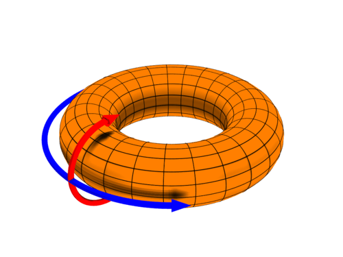
The OED also records the later usage of these terms in the context of toroidally confined plasmas, as encountered in magnetic confinement fusion. In the plasma context, the toroidal direction is the long way around the torus, the corresponding coordinate being denoted by z in the slab approximation or \(\zeta\) or \(\phi\) in magnetic coordinates; the poloidal direction is the short way around the torus, the corresponding coordinate being denoted by y in the slab approximation or \(\theta\) in magnetic coordinates. (The third direction, normal to the magnetic surfaces, is often called the “radial direction”, denoted by x in the slab approximation and variously \(\psi\), \(\chi\), r, \(\rho\), or \(s\) in magnetic coordinates.)

In vector calculus, a topic in pure and applied mathematics, a poloidal–toroidal decomposition is a restricted form of the Helmholtz decomposition. It is often used in the spherical coordinates analysis of solenoidal vector fields, for example, magnetic fields and incompressible fluids.

For a three-dimensional vector field \(\mathbf{F}\) with zero divergence

\[ \nabla\cdot\mathbf{F}=0 \]

This \(\mathbf{F}\) can be expressed as the sum of a toroidal field \(\mathbf{T}\) and poloidal vector field \(\mathbf{P}\)

\[ \mathbf{F} = \mathbf{T}+\mathbf{P} \]

where \(\widehat{r}\) is a radial vector in spherical coordinates \((r,\theta,\phi)\). The toroidal field is obtained from a scalar field, \(\psi(r,\theta,\phi)\) as the following curl,

\[ \mathbf{T}=\nabla\times(\widehat{r}\Psi(\mathbf{r})) \]

and the poloidal field is derived from another scalar field \(\phi(r,\theta,\phi)\) as a twice-iterated curl,

\[ \mathbf{P}=\nabla\times\nabla\times(\widehat{r}\Phi(\mathbf{r})) \]

This decomposition is symmetric in that the curl of a toroidal field is poloidal, and the curl of a poloidal field is toroidal. The poloidal–toroidal decomposition is unique if it is required that the average of the scalar fields \(\Psi\) and \(\Phi\) vanishes on every sphere of radius \(r\).

3.8 Magnetic Dipole Field

If there’s no current, \[ \nabla\times\mathbf{B}=\mu_0 \mathbf{J} = 0 \Rightarrow B=-\nabla V \]

The divergence free condition for magnetic field then yields a laplace equation \[ \Delta V = 0 \] for the Gauss potential \(V\). The general complex solution of Laplace equation in spherical coordinates is \[ \begin{aligned} V(\mathbf{r}) &= \sum_{l=0}^{\infty}\sum_{m=-l}^{l} \left( A_l r^l + B_l r^{-l-1} \right)P_l^m(\cos\theta)e^{-im\phi} \\ &= \sum_{l=0}^{\infty}\sum_{m=-l}^{l} \left( A_l r^l + B_l r^{-l-1} \right) Y_l^m(\theta, \phi) \end{aligned} \] where \[ Y_l^m(\theta,\phi) = P_l^m(\cos{\theta})e^{-im\phi} \] are the (complex) spherical harmonics. The indices l and m indicate degree and order of the function. The general real solution is \[ V(\mathbf{r}) = \sum_{l=0}^{\infty}\sum_{m=0}^{l} \left( A_l r^l + B_l r^{-l-1} \right)P_l^m(\cos\theta)\left[ S_m\sin{m\phi} + C_m\cos{m\phi} \right] \]

\(P_l^m\) are the associated Legendre polynomials. The first three terms of \(P_l^m(\cos\theta)\) are \[ \begin{aligned} P_0^0(\cos\theta) &= 1 \\ P_1^0(\cos\theta) &= \cos\theta \\ P_1^1(\cos\theta) &= -\sin\theta \end{aligned} \]

There are two parts in the real solution. The first part, starting with coefficients \(A_l\), represents the potential from an exterior source, which is analytic at \(r=0\) but diverges as \(r\rightarrow\infty\). The second part, starting with coefficients \(B_l\), represents the potential from an interior source, which is singular at \(r=0\) and finite as \(r\rightarrow\infty\).

Ex 1. Planet dipole field

For a planetary dipole field, we only consider the contribution from the internal source. The Gauss potential for the dipole reads \[ \begin{aligned} V &= \frac{1}{r^2}\big[ B_1C_0\cos\theta + B_1C_1\cos\phi\sin\theta + B_1S_1\sin\phi\sin\theta \big] \\ &= \frac{1}{r^2}\big[ G_{10}\cos\theta + G_{11}\cos\phi\sin\theta + H_{11}\sin\phi\sin\theta \big] \end{aligned} \]

If \(r\) is defined in the unit of planet radius, then the dipole moment \(\mathbf{m} = (G_{11},H_{11},G_{10})\) in Cartesian coordinates would have the SI unit of \([\text{T}\text{m}^3]\). We then have \[ \mathbf{B} = -\nabla V = -\nabla \Big[ \frac{\mathbf{m}\cdot\mathbf{r}}{r^3} \Big] = \frac{3(\mathbf{m}\cdot\widehat{r})\widehat{r}-\mathbf{m}}{r^3} \]

Often in literature we see dipole moments in the unit of \([\text{nT}]\,[\text{R}]^3\): this indicates that this dipole strength is equivalent to the equatorial field strength \(B_{\text{eq}}\) at the planet’s surface, and the field strength is scaled as \(r^{-3}\).

In SI units, we need to append additional coefficients \[ \mathbf{B} = \frac{\mu_0}{4\pi}\frac{3(\mathbf{m}\cdot\widehat{r})\widehat{r}-\mathbf{m}}{r^3} \] such that the dipole moment \(\mathbf{m}\) has the unit of \([\mathrm{A}]\,[\mathrm{m}]^2\), consistent with its physical meaning originated from a closed current loop.

In spherical coordinates \((r,\theta,\varphi)\) aligned with the dipole moment, \[ \mathbf{B} = \frac{\mu_0}{4\pi} \frac{m}{r^3} (-2\cos\theta, -\sin\theta, \,0) \tag{3.4}\]

It is usually convenient to work in terms of the latitude, \(\vartheta = \pi/2 - \theta\), rather than the polar angle, \(\theta\). An individual magnetic field-line satisfies the equation \[ r = r_\mathrm{eq}\,\cos^2\vartheta \] where \(r_\mathrm{eq}\) is the radial distance to the field line in the equatorial plane (\(\vartheta=0^\circ\)). It is conventional to label field lines using the L-shell parameter, \(L=r_\mathrm{eq}/R_E\). Here, \(R_E = 6.37\times 10^6\,\mathrm{m}\) is the Earth’s radius. Thus, the variation of the magnetic field-strength along a field line characterized by a given \(L\)-value is \[ B = \frac{B_E}{L^3} \frac{(1+3\,\sin^2\vartheta)^{1/2}}{\cos^6\vartheta} \] where \(B_E= \mu_0 M_E/(4\pi\, R_E^{~3}) = 3.11\times 10^{-5}\,\mathrm{T}\) is the equatorial magnetic field-strength on the Earth’s surface.

In Cartesian representation, \[ \mathbf{B} = \frac{\mu_0}{4\pi}\frac{1}{r^5} \begin{pmatrix} (3x^2-r^2) & 3xy & 3xz \\ 3yx & (3y^2-r^2) & 3yz \\ 3zx & 3zy & (3z^2-r^2) \end{pmatrix} \mathbf{m} \tag{3.5}\]

Note that \((x,y,z)\) and \(r\) are all normalized to the radius of the planet \(R\).

Ex 2. 2D dipole field

Let us consider the solution to the Laplace equation in polar coordinates \((r, \theta)\). Via separation of variable it can be shown that the general real solution takes the form \[ V = c_0\ln{r} + D_0 + \sum_{n=1}^\infty \left( A_n\cos{n\theta} + B_n\sin{n\theta} \right)\left( C_n r^n + D_n r^{-n} \right) \]

For a dipole field, we only consider \(n=1\) from the internal source. If we absorb \(D_1\) into \(A_1\) and \(B_1\), we have \[ V = (A_1\cos\theta + B_1\sin\theta)\frac{1}{r} = \frac{\mathbf{m}\cdot\mathbf{r}}{r^2} \] where the 2D magnetic moment is \(\mathbf{m}=(A_1, B_1)\).

Thus \[ \mathbf{B}_\mathrm{dipole,2D} = -\nabla V = \frac{2(\mathbf{m}\cdot\hat{r})\hat{r} - \mathbf{m}}{r^2} \tag{3.6}\] where the minus sign has been absorbed into the coefficients. 2D dipole scales as \(r^{-2}\).

Ex 3. Magnetic monopoles

Even though magnetic monopoles have not yet been observed in nature, there are some nice math tricks that allow us to approximate the magnetic dipole field as two opposite charged magnetic monopoles sitting close to each other. In 3D, the magnetic monopole would give a magnetic field \[ \mathbf{B}(\mathbf{r}) = \frac{\mu_0}{4\pi}\frac{g}{r^2}\hat{r} \] where \(g\) is the strength of the magnetic monopole in units of magnetic charge. In 2D, it would be \[ \mathbf{B}(\mathbf{r}) = C\frac{g}{r}\hat{r} \]

The analogy can be make from Coulomb’s law: an electric dipole field in 3D scales as \(r^{-3}\) when the electric monopole field scales as \(r^{-2}\).

3.9 Green’s Function

The Vlasov theory and the 2-fluid theory only tell us when instability will happen, but neither tell us the severity of instability. To know the magnitude of instability mathematically, we can introduce Green’s function \[ G(x,t)=\frac{1}{2\pi}\int_{-\infty}^{\infty}e^{ikx-i\omega(k) t}dk \] where \(t\) is the beam’s pulse length and \(x\) is the propagation distance. At \(t=0\), we have \[ \begin{aligned} G(x,0)&=\frac{1}{2\pi}\int_{-\infty}^{\infty}e^{ikx}dk=\frac{1}{2i\pi x}e^{ikx}\bigg|_{k=-\infty}^{k=\infty} \\ &=\lim_{k\rightarrow\infty}\frac{1}{2i\pi x}\big[ \cos{kx}+i\sin{kx}-\cos{kx}+i\sin{kx} \big] \\ &=\lim_{k\rightarrow\infty}\frac{1}{\pi}\frac{\sin{kx}}{x}=\delta(x) \end{aligned} \] where \(\delta(x)\) is the \(\delta\)-function.

The integral \(\int_0^{\infty}\frac{\sin x}{x}\mathrm{d}x\) is called the Dirichlet integral. It is a very famous and important generalized improper integral. Here at least you can see that \[ \int_{-\infty}^{\infty}G(x,0)=\frac{1}{\pi}\int_0^\infty \frac{\sin kx}{x}\mathrm{d}x=1\quad \textrm{and}\quad G(0,0)=\infty \]

3.10 Linearization

In linear wave analysis, we need to check how small perturbations evolve in the PDEs. For plasma physics, it is usually very useful to transform into a magnetic field guided coordinates, with the notation \(\parallel\) being parallel to the background magnetic field and \(\perp\) being perpendicular to the background magnetic field \(\mathbf{B}\). Besides the perturbation of plasma moments (i.e. density, velocity, pressure, etc.), we also need the perturbations to the magnitude of the magnetic field B and the unit vector \(\hat{\mathbf{b}}\). Linearzing \(B^2 = \mathbf{B}\cdot\mathbf{B}\), we find \[ \delta B = \hat{\mathbf{b}}\cdot\delta\mathbf{B} = \delta B_\parallel \tag{3.7}\]

Linearzing \(\hat{\mathbf{b}} = \mathbf{B}/B\), we obtain \[ \begin{aligned} \delta\hat{\mathbf{b}} = \delta\left(\frac{\mathbf{B}}{B}\right) = \frac{\delta\mathbf{B}B - \delta B\mathbf{B}}{B^2} = \frac{\delta\mathbf{B}}{B} - \frac{\delta \mathbf{B}_\parallel}{B} = \frac{\delta \mathbf{B}_\perp}{B} \end{aligned} \tag{3.8}\]

The divergence-free of magnetic field gives \[ \mathbf{k}\cdot\delta\mathbf{B} = k_\parallel \delta B_\parallel + k_\perp \delta B_\perp = 0 \]

Thus \[ \mathbf{k}\cdot\hat{\mathbf{b}} = \mathbf{k}\cdot\frac{\delta \mathbf{B}_\perp}{B} = \frac{k_\perp \delta B_\perp}{B} = -k_\parallel\frac{\delta B_\parallel}{B} = -k_\parallel\frac{\delta B}{B} \tag{3.9}\]

These seemingly trivial relations have profound implications in physics. Equation 3.7 tells us that the perturbation of magnetic field magnitude has only contribution from the parallel component, which is why in satellite observations people only look at parallel perturbations for compressional wave modes. Equation 3.8 tells us that the perturbation in the unit vector is only related to the perpendicular fluctuations.

3.11 Wave Equations

The waves in plasma physics is governed by second order ODEs. Here we list some second order ODEs that has been studied mostly in plasma physics.

• Schrödinger Equation:

\[ \frac{\mathrm{d}^2\varphi}{\mathrm{d}x^2} + \frac{2m}{\hbar^2}\big[ E-U(x)\big]\varphi= 0 \]

Schrödinger Equation appears in the nonlinear wave studies (Chapter 14).

• Shear Alfvén wave:

\[ \frac{\mathrm{d}}{\mathrm{d}x}\Big\{ \rho_0 \big[ \omega^2 - (\mathbf{k}\cdot\mathbf{v}_A(x))^2 \big]\frac{dE}{\mathrm{d}x} \Big\} - k^2\rho_0 \big[ \omega^2 - (\mathbf{k}\cdot\mathbf{v}_A)^2 - g\frac{1}{\rho_0}\frac{\mathrm{d}\rho_0}{\mathrm{d}x} \big]E = 0 \]

The Shear Alfvén wave equation appears in nonuniform ideal MHD (Equation 7.30, Equation 13.8).

• EM waves in non-magnetized plasma, O mode:

\[ \frac{\mathrm{d}^2 E}{\mathrm{d}x^2} + \frac{\omega^2}{c^2} \Big[ 1-\frac{{\omega_{pe}(x)}^2}{\omega^2} \Big]E = 0 \tag{3.10}\]

• Electron cyclotron resonance heating (ECRH):

\[ \frac{\mathrm{d}^2 E}{\mathrm{d}x^2} + \frac{\omega^2}{c^2} \Big[ 1-\frac{{\omega_{pe}(x)}^2}{\omega(\omega-\Omega_e(x))} \Big]E = 0 \]

In general, a second order ODE \[ \frac{\mathrm{d}^2 u(x)}{\mathrm{d}x^2} + a_1(x)\frac{du(x)}{\mathrm{d}x} + a_2(x)u(x) = 0 \] can be rewritten to get rid of the first derivative. Let \[ u(x) = E(x) e^{-\frac{1}{2}\int^x a_1(x)\mathrm{d}x} \] we have \[ \frac{\mathrm{d}^2 E(x)}{\mathrm{d}x^2} + k^2(x) E(x) = 0 \tag{3.11}\] where \[ k^2(x) = a_2(x) - \frac{{a_1}^2}{4} -\frac{1}{2}\frac{\mathrm{d} a_1(x)}{\mathrm{d}x} \]

Note that the lower bound of the integral is left on purpose to account for a constant. We will concentrate at special points, i.e. zeros (cutoff) and poles (resonance) of \(k^2(x)\equiv \frac{\omega^2}{c^2}n^2(x)\).

First, we will introduce Wentzel–Kramers–Brillouin-Jeffreys (WKBJ) solution to Equation 3.11: \[ E(x) \sim \frac{1}{\sqrt{k(x)}}e^{\pm i\int^x k(x^\prime)\mathrm{d}x^\prime}. \]

Proof.

For simplicity, here we use a simple harmonic oscillation analogy. Consider \[ \frac{\mathrm{d}^2 x(t)}{\mathrm{d}t^2} + \Omega^2(t)x(t) = 0 \]

Assume \(\Omega \gg 1\), and \(T\) is the time scale over which \(\Omega\) changes appreciably. We would anticipate solutions like \[ \begin{aligned} &x(t)\sim e^{\pm i \Phi(t)} \\ &\dot{x}(t) \sim \pm i \dot{\Phi}(t) x(t) \\ &\ddot{x}(t) \sim - \dot{\Phi}^2(t) x(t) \cancel{\pm i \ddot{\Phi}(t)x(t)} \\ \Rightarrow &\dot{\Phi}(t) = \Omega(t),\ \text{or } \Phi(t) = \int^t \Omega(t^\prime) \mathrm{d}t^\prime + \text{const.} \end{aligned} \]

Write \(x(t) = A(t)\sin{[\Phi(t)]}\), where \(A(t)\) is slowly varying in time, \(\dot{A}(t)\ll \Omega A\), which is almost a periodic motion. From adiabatic theory in classical mechanics, \(\oint pdq \simeq \text{const.}\), we have \[ \begin{aligned} \oint mv_x \mathrm{d} x \simeq \text{const.} \\ \oint m\dot{x}\dot{x}\mathrm{d}t \simeq \text{const.} \end{aligned} \]

Then in a period \(2\pi/\Omega\), \[ \frac{2\pi}{\Omega}\oint m\dot{x}^2dt =\frac{2\pi}{\Omega}\oint mA^2 \Omega^2\cos^2\Phi \mathrm{d}t \simeq \text{const.} \] which leads to \[ mA^2\Omega \simeq \text{const.},\ A\sim\frac{1}{\sqrt{\Omega}} \]

Thus the general form of solution can be written as \[ x(t)\sim\frac{1}{\sqrt{\Omega}}e^{\pm i \Phi(t)} \sim\frac{1}{\sqrt{\Omega}} e^{\pm i \int^t \Omega(t^\prime)\mathrm{d}t^\prime+\text{const.}} \]

□

Note:

1. There is no lower limit to the integral, because it is like adding a constant.
2. This solution is valid if \(k\cdot L > O(3)\), where \(L\) is the length scale over which \(k^2(x)\) changes appreciably. (???)Formally the condition should be \(kL\gg 1\). Apparently near resonance (\(k\rightarrow\infty\)), the condition breaks down, then how do we reconcile the solution? There are more discussions coming up and applications in Chapter 7 and Chapter 13.

3.11.1 Airy Function

We want to develop a general method for cut-off and resonance. Away from the turning point \(x_t\), \[ E_{\text{WKBJ}}(x) \sim \frac{1}{\sqrt{k(x)}}e^{\pm i\int^x k(x)\mathrm{d}x} \]

Near \(x=x_t\), we can use a linear approximation for \(k^2(x)\) (first term in the Taylor expansion), \[ k^2(x) \approx -{k_0}^2 a(x-x_t) \]

Then \[ \begin{aligned} \frac{\mathrm{d}^2 E}{\mathrm{d}x^2} + k^2(x)E &= 0 \\ \frac{\mathrm{d}^2 E}{\mathrm{d}x^2} - {k_0}^2 a (x-x_t) E &= 0 \end{aligned} \]

Let \(\frac{x-x_t}{l}=\zeta\), we have \[ \frac{\mathrm{d}^2 E}{\mathrm{d}\zeta^2} - l^2 {k_0}^2 a l \zeta E(\zeta) = 0 \]

If we choose \(l\) s.t. \(l^3 {k_0}^2 a =1\) (non-dimensional treatment), we obtain \[ \frac{\mathrm{d}^2 E}{\mathrm{d}\zeta^2} - \zeta E(\zeta) = 0 \tag{3.12}\]

which is equivalent to the case where \(k^2(\zeta)=-\zeta\) that shows the linear approximation. Equation 3.12, known as the Airy equation or Stokes equation, is the simplest second-order linear differential equation with a turning point (a point where the character of the solutions changes from oscillatory to exponential). From the WKBJ theory, we get the solution \[ E_{\text{WKBJ}} \sim \frac{1}{\sqrt{k(x)}}e^{\pm i\int^x k(x^\prime)\mathrm{d}x^\prime} = \left\{ \begin{array}{rl} \zeta^{-1/4}e^{\mp\frac{2}{3}\zeta^{3/2}} & \text{if } \zeta > 0 \\ (-\zeta)^{-1/4}e^{\pm i \frac{2}{3}(-\zeta)^{3/2}} & \text{if } \zeta < 0 \end{array} \right. \]

Note that the solution blows up at \(\zeta=0\) (turning point) miserably. For \(\zeta>0\), one solution is exponentially decay while the other is exponentially growing; for \(\zeta<0\), the two solutions are oscillatory. Solutions can also be found as series in ascending powers of \(\zeta\) by the standard method. Assume that a solution is \(E=a_0+a_1\zeta+a_2\zeta^2+...\) Substitute this in Stokes Equation and equate powers of \(\zeta\) will give relations between the constants \(a_0,a_1,a_2\),etc., and lead finally to \[ \begin{aligned} E = &a_0\Big\{ 1+\frac{\zeta^3}{3\cdot2} +\frac{\zeta^6}{6\cdot5\cdot3\cdot2} + \frac{\zeta^9}{9\cdot8\cdot6\cdot5\cdot3\cdot2} + ... \Big\} \\ &+a_1\Big\{ \zeta+\frac{\zeta^4}{4\cdot3} +\frac{\zeta^7}{7\cdot6\cdot4\cdot3} + \frac{\zeta^{10}}{10\cdot9\cdot7\cdot6\cdot4\cdot3} + ... \Big\} \end{aligned} \] which contains the two arbitrary constants \(a_0\) and \(a_1\), and is therefore the most general solution. The series are convergent for all \(\zeta\), which confirms that every solution of Stokes Equation is finite, continuous and single valued.

This form is usually not easy to interpret in physical sense. Besides this, we can find a more useful solution to Equation 3.12 using the integral representation. An equivalent but maybe more intuitive approach is to solve Equation 3.12 with Fourier transform; a coefficient \(2\pi\) naturally appears. Both approaches reach the same results.

Write \[ E(\zeta) = \int_a^b \mathrm{d}t e^{t\zeta} f(t) \] where the integral represents a path in the complex t plane from \(a\) to \(b\). Then \[ \begin{aligned} \frac{\mathrm{d}^2 E}{\mathrm{d}\zeta^2} &= \int_a^b \mathrm{d}t\ t^2 e^{t\zeta} f(t) \\ \zeta E(\zeta) &= \int_a^b \mathrm{d}t \zeta e^{t\zeta} f(t) = \int_a^b \mathrm{d}t \frac{\mathrm{d}}{\mathrm{d}t}(e^{t\zeta}) f(t) \\ &=e^{t\zeta} f(t) \Big|_a^b -\int_a^b dte^{t\zeta} f^\prime(t) \end{aligned} \]

The limits \(a,b\) are be chosen so that the first term vanishes at both limits. Then Equation 3.12 is satisfied if

\[ \left\{ \begin{array}{l} e^{t\zeta} f(t) \Big|_a^b = 0\\ t^2 f(t) = -\frac{\mathrm{d} f(t)}{\mathrm{d}t} \Rightarrow f(t) = Ae^{-\frac{1}{3}t^3} \end{array} \right. \]

where \(A\) is a constant. The solution is now written as

\[ E(\zeta) = \int_a^b \mathrm{d}t Ae^{t\zeta-\frac{1}{3}t^3} \]

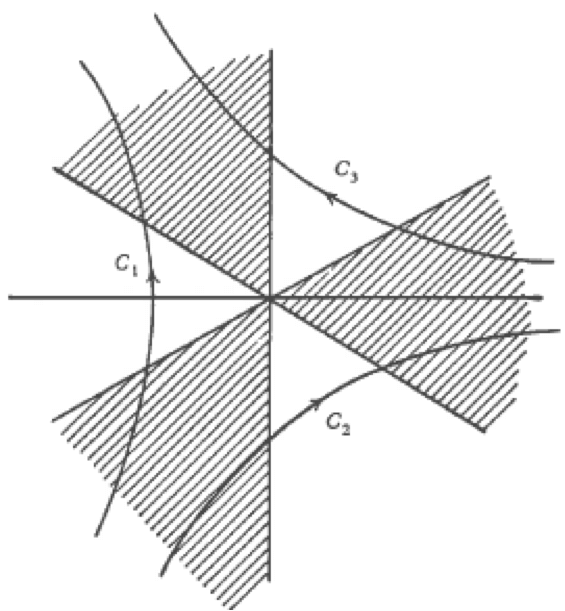
The limits \(a\) and \(b\) must therefore be chosen so that \(e^{t\zeta-\frac{1}{3}t^3}\) is zero for both. (Note that \(\zeta\) is a constant.) This is only possible if \(t=\infty\) and the real part of \(t^3\) is positive:

\[ \begin{aligned} \Re(t^3) > 0 \Leftrightarrow 2\pi n -\frac{1}{2}\pi < \arg{t^3} < 2\pi n + \frac{1}{2}\pi \\ \Leftrightarrow 2\pi n -\frac{1}{2}\pi < 3 \arg{t} < 2\pi n + \frac{1}{2}\pi \end{aligned} \]

where \(n\) is an integer. Figure 3.2 is a diagram of the complex t-plane, and \(a\) and \(b\) must each be at \(\infty\) in one of the shaded sectors. They cannot both be in the same sector, for then the integral would be zero. Hence the contour may be chosen in three ways, as shown by the three curves \(C_1,C_2,C_3\), and the solution would be

\[ E(\zeta) = \int_{C_1,C_2,C_3} \mathrm{d}t\ e^{t\zeta-\frac{1}{3}t^3} \]

This might appear at first to give three independent solutions, but the contour \(C_1\) and be distorted so as to coincide with the two contours \(C_2+C_3\), so that

\[ \int_{C_1} = \int_{C_2} + \int_{C_3} \]

and therefore there are only two independent solutions.

Figure 3.2: Solution to Stokes Equation in complex t-plane.

Proof.

Note that:

1. \(e^{A}\neq 0\ \forall |A|<\infty\);
2. \(e^{A}=0 \Leftrightarrow\, A\rightarrow \infty\,\text{and}\,\Re(A)<0\).

Therefore we have

\[ e^{-\frac{1}{3}t^3}\rightarrow 0\,\text{as}\, t\rightarrow \infty\,\text{and}\,\Re\Big(\frac{1}{3}t^3\Big)>0 \] In polar coordinates, let \(t=|t|e^{i\theta}\). Then

\[ t^3 = |t|^3 e^{i3\theta} = |t|^3 \big( \cos{3\theta} + i\sin{3\theta} \big) \]

\[ \Re\Big(\frac{1}{3}t^3\Big)>0 \iff \cos{3\theta}>0 \iff 3\theta \in (-\frac{\pi}{2},\frac{\pi}{2}),\ (\frac{3\pi}{2},\frac{5\pi}{2}),\ (-\frac{3\pi}{2},-\frac{5}{2}\pi) \]

□

Jeffreys (1956) defines two special Airy functions \(Ai(x), Bi(x)\) as follows

\[ \begin{aligned} Ai(\zeta) &= \frac{1}{2\pi i}\int_{C_1} \mathrm{d}t e^{-\frac{1}{3}t^3 + \zeta t} \\ Bi(\zeta) &= \frac{1}{2\pi} \Big[\int_{C_2}+\int_{C_3}\Big]\mathrm{d}t e^{-\frac{1}{3}t^3 + \zeta t} \end{aligned} \tag{3.13}\]

Obviously he took the Fourier transform such that a coefficient \(2\pi\) naturally appears. In Equation 3.13, the contour \(C_1\) can be distorted so as to coincide with the imaginary t-axis for almost its whole length. It must be displaced slightly to the left of this axis at its ends to remain in the shaded region at infinity. Let \(t=is\). Then the Airy function of the first kind in Equation 3.13 becomes

\[ \begin{aligned} Ai(\zeta) &= \frac{1}{2\pi}\int_{-\infty}^{\infty}e^{i(\zeta s+\frac{1}{3}s^3)}ds \\ &=\frac{1}{\pi}\int_{0}^{\infty}\cos\Big(\zeta s+\frac{1}{3}s^3\Big)ds \end{aligned} \]

It is known as the Airy integral, which is the solution for \(y\rightarrow 0\) as \(x\rightarrow\infty\). The other linearly independent solution, the Airy function of the second kind, denoted \(Bi(x)\), is defined as the solution with the same amplitude of oscillation as \(Ai(x)\) as \(x\rightarrow -\infty\) which differs in phase by \(\pi/2\):

\[ Bi(\zeta) = \frac{1}{\pi}\int_{0}^{\infty}\Big[e^{-\frac{s^3}{3}+s\zeta} + \sin\Big(\zeta s+\frac{1}{3}s^3\Big)\Big]ds \]

\(Ai(x)\) and \(Bi(x)\) are shown in ?fig-airy.

KeyNotes.plot_airy()

As an interesting experiment, we can check if \(Ai(x)\) is recovered from solving the second order ODE numerically:

@sco KeyNotes.plot_airy_ode()

Here we start from the right boundary and move towards the left.

Now, to find approximations for Airy functions, we use the method of steepest descent. This approximation is based on the assumption that major contribution to the integral is from near the saddle point. As an example of saddle point, consider a complex function \(\exp{f(z)}=e^{-z^2}\), where \(z=x+i y\).

• If \(z=\text{real} = x\), \(e^{-z^2}=e^{-x^2}\);
• If \(z=\text{imag}=iy\), \(e^{-z^2}=e^{y^2}\).

The procedure goes as follows:

1. Detour path of integral s.t. it passes through the saddle point of the integral, along the direction of steepest descent.
2. Obtain major contribution by integrating the Gaussian function.

\[ I=\int_C \mathrm{d}t e^{f(t)},\quad f(t) = f(t_s) + (t-t_s)f^\prime(t_s) + \frac{1}{2}(t-t_s)^2 f^{\prime\prime}(t_s) + ... \] where \(f^\prime(t_s)=0\) at the saddle point \(t=t_s\) simplifies \(I\) to the integral of a Gaussian function.

For \(Ai(\zeta)\), \[ \begin{aligned} f(t) &= t\zeta -\frac{1}{3}t^3 \\ f^\prime(t_s)& = \zeta - {t_s}^2 = 0 \\ f^{\prime\prime}(t_s)& = -2t_s \end{aligned} \]

Consider \(\zeta>0\) (where the solution is either exponentially decaying or growing.) Then \[ \begin{aligned} t_{s1} = -\sqrt{\zeta},\quad t_{s2} = \sqrt{\zeta} \\ f(t_{s1}) = -\frac{2}{3}\zeta^{3/2},\quad f^{\prime\prime}(t_{s1}) = 2\zeta^{1/2} \end{aligned} \] So \[ \begin{aligned} Ai(\zeta) &= \frac{1}{2\pi i} \int_{C_1} \mathrm{d}t\ e^{-\frac{2}{3}\zeta^{3/2}+\zeta^{1/2}(t-t_s)^2}+... \\ &\approx\frac{1}{2\pi i} e^{-\frac{2}{3}\zeta^{3/2}}\int_{C_1}\mathrm{d}t\ e^{\sqrt{\zeta}(t-t_s)^2} \end{aligned} \]

Let \(e^{\sqrt{\zeta}(t-t_s)^2}=e^{-\rho^2}\), where \(\rho=\text{real}\) is the direction of steepest descent, and \(\rho=\text{imag}\) is the direction of steepest ascent.

\[ \begin{aligned} i\rho &= \pm \zeta^{1/4} (t-t_s) \\ \mathrm{d}t&=\frac{i \mathrm{d}\rho}{\zeta^{1/4}} \Rightarrow\ \mathrm{d}t \text{ is purely imaginary along steepest descent.} \end{aligned} \]

Then for \(\zeta>0\) \[ \begin{aligned} Ai(\zeta) &= \frac{1}{2\pi i}e^{-\frac{2}{3}\zeta^{3/2}}\int_{-\infty}^{\infty}\frac{id\rho}{\zeta^{1/4}}e^{-\rho^2} \nonumber \\ &=\frac{1}{2\sqrt{\pi}\zeta^{1/4}}e^{-\frac{2}{3}\zeta^{3/2}} \text{ as}\ \zeta\rightarrow \infty \end{aligned} \tag{3.14}\]

The ratio of accuracy is shown in the following table (LABEL???). In practice, it is already a very good approximation when \(\zeta>3\). (think of \(kL\gg 3\) for WKBJ solution! ???)

\(\zeta\)	1	2	3	6	\(\infty\)
ratio	0.934	0.972	0.983	0.993	1

Now, consider \(\zeta<0\). When \(\zeta\rightarrow-\infty\), we anticipate oscillating behavior of \(Ai(\zeta)\). \(\zeta=-|\zeta|\), \[ \begin{aligned} &\left\{ \begin{array}{rl} f(t) &= \zeta t-\frac{1}{3}t^3 = -t|\zeta| - \frac{1}{3}t^3 \\ f^\prime(t) &= -|\zeta| - t^2 = 0 \\ f^{\prime\prime}(t) &= -2t \end{array} \right. \\ \Rightarrow &f(t_{s1}) = i\frac{2}{3}|\zeta|^{3/2} \\ &f^{\prime\prime}(t_{s1}) = 2i\sqrt{|\zeta|} \end{aligned} \] so the contribution from \(t_{s1}\) is \[ \frac{1}{2\pi i}e^{i\frac{2}{3}|\zeta|^{3/2}}\int_{t_{s1}} e^{\frac{1}{2}(2i\sqrt{|\zeta|})(t-t_s)^2+...} \]

Let \(-\rho^2=i\sqrt{|\zeta|}(t-t_{s1})^2\), differentiate on both sides to get \[ \mathrm{d}t = \pm\frac{e^{i\pi/4}}{|\zeta|^{1/4}}\mathrm{d}\rho \]

Again, \(\rho=\text{real}\) is the direction of steepest descent at \(t=t_{s1}\). Do the same to \(t_{s2}\), then by summing them up we have for \(\zeta<0\), \[ \begin{aligned} Ai(\zeta) &\approx \frac{1}{2\pi i} \Big[ e^{i\frac{2}{3}|\zeta|^{3/2}}\int_{-\infty}^{\infty}\frac{e^{i\pi/4}}{|\zeta|^{1/4}}\mathrm{d}\rho e^{-\rho^2} - e^{-i\frac{2}{3}|\zeta|^{3/2}}\int_{-\infty}^{\infty}\frac{e^{-i\pi/4}}{|\zeta|^{1/4}}\mathrm{d}\rho e^{-\rho^2} \Big] \\ &= \frac{1}{2\pi i} \Big[ \frac{e^{i\frac{2}{3}|\zeta|^{3/2}+i\pi/4}}{{|\zeta|^{1/4}}} \sqrt{\pi} - \frac{e^{-i\frac{2}{3}|\zeta|^{3/2}-i\pi/4}}{{|\zeta|^{1/4}}} \sqrt{\pi} \Big] \end{aligned} \tag{3.15}\]

An interesting application of the gradient descent method is to find Stirling’s approximation. Mathematically, we can proof that \[ n! =\int_0^\infty \mathrm{d}t\ e^{-t}t^n = \int_0^\infty \mathrm{d}t\ e^{-t+n\ln{t}} \equiv \int_0^\infty \mathrm{d}t\ e^{f(t)} \] and by following the steepest descent method, \[ \begin{aligned} f(t) &= -t +n\ln{t} \\ f^\prime(t) &= -1 + n\frac{1}{t}=0 \\ f^{\prime\prime}(t) &= -n\frac{1}{t^2} \end{aligned} \]

we can find the approximation Stirling formula \[ \begin{aligned} n! &\approx \int_0^\infty \mathrm{d}t\ e^{-n+n\ln{n}-\frac{1}{2n}(t-t_s)^2} \\ &=e^{-n}n^n \int_0^\infty \mathrm{d}t\ e^{-\frac{1}{2n}(t-t_s)^2} \\ &=\sqrt{2n\pi}e^{-n}n^n \end{aligned} \]

The following table (LABEL???) show the goodness of approximation of Stirling formula. In practice, it is already a very good approximation when \(n>3\).

\(\zeta\)	1	2	3	10	\(\infty\)
ratio	0.922	0.9595	0.973	0.9917	1

See (Budden 1961) Chapter 15: The Airy Integral Function, And The Stokes Phenomenon for more details.

3.11.2 Uniformly Valid WKBJ Solution Across the Turning Point

In this section, we present the WKBJ solution that is uniformly valid everywhere, even at the turning point.

Consider the standard equation,

\[ \frac{\mathrm{d}^2E(x)}{\mathrm{d}x^2}+k^2(x)E(x) = 0 \]

Let \(x=0\) be the turning point, i.e. we assume that \(k^2(x)\) is a monotonically decreasing function of \(x\) with \(k(0)=0\). For the region \(x>0\), we first identify the exponentially decaying factor of the Airy function, \(Ai(\zeta)\), to be the phase integral in the WKBJ solution:

\[ -\frac{2}{3}\zeta^{3/2} = i \int_0^x k(x^\prime)\mathrm{d}x^\prime \]

Note that this yields \(\zeta=\zeta(x)\), a known function of x (I confuse myself later about \(\zeta\) and \(x\)…). The branch for \(\zeta(x)\) is to be chosen so that for \(x>0\), \(\zeta\) is real and positive.

We next verify that the uniformly valid solution to the standard equation is simply

\[ E(x) = \frac{1}{\sqrt{\zeta^\prime(x)}}Ai(\zeta) \tag{3.16}\]

where the prime denotes a derivative. For large values of \(\zeta\), we can use the asymptotic formula of \(Ai\) Equation 3.14, and notice that

\[ \begin{aligned} -\zeta^{1/2}\zeta^\prime = ik(x) \\ \zeta^\prime(x) = -i \frac{k(x)}{\zeta^{1/2}} \end{aligned} \]

we can see that Equation 3.16 reduces to the standard WKBJ solutions for large values of \(\zeta\)

\[ E(x)= \frac{1}{\sqrt{\zeta^\prime(x)}}Ai(\zeta) \sim \frac{1}{\sqrt{k(x)}} e^{-\frac{2}{3}\zeta^{3/2}} = \frac{1}{\sqrt{k(x)}}e^{ i \int_0^x k(x^\prime)\mathrm{d}x^\prime} \]

We can also show that Equation 3.16 is valid for small values of \(\zeta\), i.e. near the turning point at \(x=0\). (Hint: Near \(x=0\), \(k^2(x)\) may be approximated by a linear function of \(x\). This linear approximation then yields \(\zeta(x)\) as a linear function of \(x\) according to Equation 3.16.)

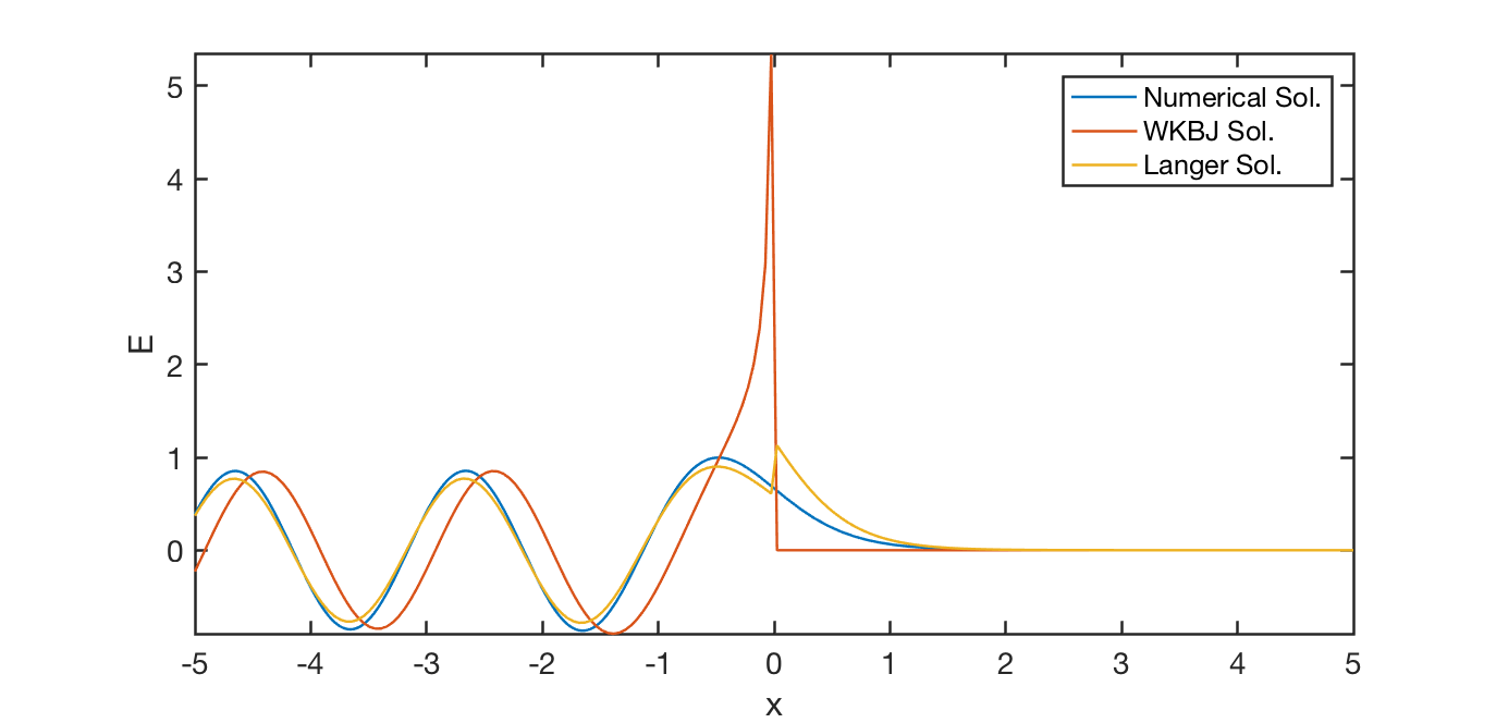
Ex. Choose a smooth plasma density profile which monotonically increases with \(x\) s.t.

\[ \frac{\omega_{pe}^2(x)}{\omega^2} = 1 + \tanh{x} \]

and launch a wave of frequency \(\omega\) from \(x=-\infty\), the vacuum region, toward the positive \(x\)-direction with \(\frac{\omega^2}{c^2} = 10 \text{m}^{-2}\). (This is like launching a wave from low \(B\) region into high \(B\) region.) Numerically integrate the wave equation Equation 3.10,

\[ \frac{\mathrm{d}^2 E}{\mathrm{d}x^2} + \frac{\omega^2}{c^2} \Big[ 1-\frac{{\omega_{pe}(x)}^2}{\omega^2} \Big]E = 0 \]

from some large positive values of \(x\), we get the results in Figure 3.3.

Figure 3.3: Comparison between the WKBJ solution, uniformly valid solution and numerical integral solution for the O-mode with monotonically increasing density with \(x\).

We know that away from \(x_t\), WKBJ solution works. To the left of \(x_t\) (with \(\zeta<-3\)), Equation 3.15 gives

\[ Ai(\zeta) = \frac{1}{2i\sqrt{\pi}|\zeta|^{1/4}}\Big[ e^{i \frac{2}{3}|\zeta|^{3/2}+i\frac{\pi}{4}} - e^{-\frac{2}{3}|\zeta|^{3/2}-i\frac{\pi}{4}} \Big] \]

Choose the branch s.t. \(\zeta{x}>0\) if \(x>x_t\); \(\zeta(x)<0\) if \(x<x_t\).

\[ \begin{aligned} E(x) &= \frac{1}{\sqrt{\zeta^\prime(x)}}Ai(\zeta) \\ &= \frac{C_3}{\sqrt{k(x)/|\zeta|^{1/2}}}\frac{1}{|\zeta|^{1/4}}\Big\{ e^{i \frac{2}{3}|\zeta|^{3/2}+i\frac{\pi}{4}} - c.c \Big\} \\ &= \frac{C_3}{\sqrt{k(x)}}\Big\{ e^{i(-\int_{x_t}^x k(x^\prime)\mathrm{d}x^\prime)+i\frac{\pi}{4}} - c.c \Big\} \\ &=\frac{C_3}{\sqrt{k(x)}}\Big\{ e^{-i\int_{x_t}^a k(x^\prime)\mathrm{d}x^\prime - i\int_a^x k(x^\prime)\mathrm{d}x^\prime+i\frac{\pi}{4}} -c.c \Big\} \\ &=\frac{C_4}{\sqrt{k(x)}}\Big\{ e^{-i \int_a^x k(x^\prime)\mathrm{d}x^\prime}-e^{i\int_{x_t}^a k(x^\prime)\mathrm{d}x^\prime } e^{2i\int_{x_t}^a k(x^\prime)\mathrm{d}x^\prime -i\frac{\pi}{2}} \Big\} \\ &=\frac{C_4}{\sqrt{k(x)}}\Big\{ e^{-i\int_a^x k \mathrm{d}x^\prime} + R\cdot e^{i\int_a^x k \mathrm{d}x^\prime} \Big\}, \end{aligned} \]

where

\[ C_4 = C_3 \cdot e^{-i \int_{x_t}^a k \mathrm{d}x^\prime + i\frac{\pi}{4}} \]

and

\[ R = -e^{2i\int_{x_t}^a k \mathrm{d}x^\prime - i\frac{\pi}{2}} = i e^{2i\int_{x_t}^a k \mathrm{d}x^\prime} = i e^{-2i \int_{a}^{x_t}kdx^\prime} \]

is the reflection coefficient at \(x=a\).

3.11.3 Stokes Phenomenon

In complex analysis the Stokes phenomenon is that the asymptotic behavior of functions can differ in different regions of the complex plane, and that these differences can be described in a quantitative way.

Ex. For the simple wave equation

\[ \frac{\mathrm{d}^2 E}{dz^2} - E = 0 \]

the solution can be given in various forms

\[ \begin{aligned} E=e^z,e^{-z},\cosh{z},\sinh{z} \\ E = \cosh{z}=\frac{1}{2}(e^z+e^{-z}) \Rightarrow \left\{ \begin{array}{rl} &E\sim\frac{1}{2}e^z\, z\rightarrow\infty \\ &E\sim\frac{1}{2}e^{-z}\, z\rightarrow-\infty \end{array} \right. \\ E = \sinh{z}=\frac{1}{2}(e^z-e^{-z}) \Rightarrow \left\{ \begin{array}{rl} &E\sim\frac{1}{2}e^z\, z\rightarrow\infty \\ &E\sim\frac{-1}{2}e^{-z}\, z\rightarrow-\infty \end{array} \right. \end{aligned} \]

Note that if a solution is exponentially growing in one direction, its asymptotic solution can contain an arbitrary amount of the exponentially decaying solution; that is, specifying an asymptotic growing solution in one direction cannot completely specify the solution in the entire complex plane.

The two linearly independent approximate solutions to Airy Equation 3.12 are the Airy function approximations from WKBJ method:

\[ \begin{aligned} &\frac{\mathrm{d}^2 E}{\mathrm{d}\zeta^2} - \zeta E = 0 \\ \Rightarrow &E(\zeta) = \left\{ \begin{array}{rl} &Ai(\zeta)\sim \frac{1}{2\sqrt{\pi}\zeta^{1/4}}e^{-\frac{2}{3}\zeta^{3/2}},\quad \zeta>0 \\ &Bi(\zeta)\sim \frac{1}{2\sqrt{\pi}\zeta^{1/4}}e^{\frac{2}{3}\zeta^{3/2}},\quad \zeta>0 \end{array} \right. \\ \end{aligned} \]

which is very accurate for \(\zeta>3\) (see previous section).

Stokes found that you can add an arbitrary amount of \(Ai(\zeta)\) to \(Bi(\zeta)\) without changing the behaviour of solution. (\(Ai(\zeta)<O(\zeta^{-1})\)???)

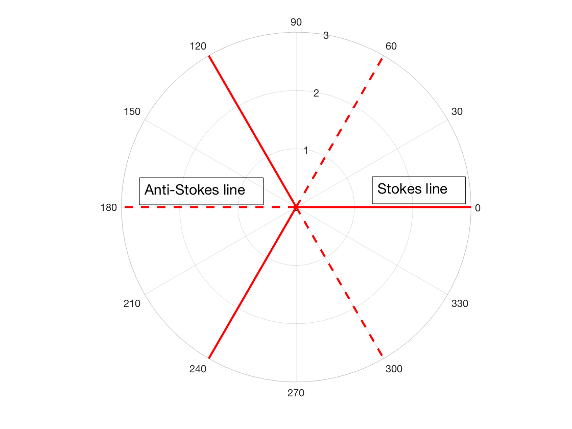
We want to find \(\zeta\) s.t. \(E_{\text{WKBJ}}\) is purely growing/decaying exponentially:

\[ \begin{aligned} \zeta^{3/2} \text{is purely real} \iff (|\zeta|e^{i\theta})^{3/2} \text{is purely real} \iff \sin{\frac{3}{2}\theta} = 0,\ \theta=0,\pm\frac{2}{3}\pi,\pm\frac{4}{3}\pi \end{aligned} \]

The lines in the complex plane on which WKBJ solution is purely growing/decaying exponentially are called Stokes lines (Figure 3.4). It is accompanied with anti-Stokes lines (in the opposite direction to Stokes lines), on which WKBJ solution is purely oscillatory. The exponentially growing solution on Stokes lines is called the dominant solution; the decaying solution on Stokes lines is called the sub-dominant/recessive solution. The sub-dominant solution will always becomes dominant in a neighboring Stokes line. However, the inverse is not true. (It may contain an amount of sub-dominant solution.) Each term changes from dominant to subdominant, or the reverse, when \(\zeta\) crosses an anti-Stokes line???

Figure 3.4: Stokes lines and anti-Stokes lines for WKBJ solution of Airy Equation.

Even though we say “arbitrary”, the analytic solution in the whole complex plane possess a limit on that amount. The next question would be: how much exponentially decaying solution can you add to the exponentially growing solution? (Note that the asympotic series is also a divergent series: more terms don’t lead to high resolution accuracy! I have questions on this part???)

For the asymptotic approximation solution of Airy Equation 3.12, we need to define \(\arg(\zeta)\) properly to make it single value. Let us choose the branch cut \(-\pi\le\arg{\zeta}<\pi\). The complex plane is demonstrated in Figure 3.5.

Figure 3.5: Marked Stokes lines and regions for Airy solution.

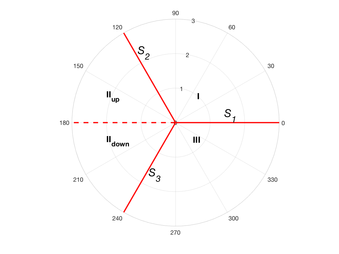
Let us start from region I. The solution in region I is

\[ E_I \sim \zeta^{-1/4}\big[ A_1 e^{-\frac{2}{3}\zeta^{3/2}} + B_1 e^{\frac{2}{3}\zeta^{3/2}}\big] \]

On \(S_1\), \(e^{-\frac{2}{3}\zeta^{3/2}}\) is sub-dominant, \(e^{\frac{2}{3}\zeta^{3/2}}\) is dominant. (The former would be dominant on neighboring Stokes lines \(S_2\) and \(S_3\).) Crossing \(S_2\) into region \(\text{II}_{\text{up}}\), we have

\[ E_{\text{II}_{\text{up}}} \sim \zeta^{-1/4} \Big[ \underbrace{A_1 e^{-\frac{2}{3}\zeta^{3/2}}}_{\text{dominant}} + \underbrace{(\lambda_1 A_1 + B_1)e^{\frac{2}{3}\zeta^{3/2}}}_{\text{sub-dominant}} \Big] \]

where \(\lambda_2\) is the Stokes constant on \(S_2\). The constant in the subdominant term has changed by \(\lambda_2 A_1\) because the differential equation is linear, and it cannot depend on \(B_1\). Otherwise it would be unaltered if we added to the solution in region I any multiple of the solution in which \(A_1=0\). (See (Budden 1961) 15.13.) Crossing the branch cut to region \(\text{II}_{\text{down}}\), \(\zeta^{\text{up}} = \zeta^{\text{down}}e^{i2\pi}\).

\[ \begin{aligned} \zeta_{\text{up}}^{-1/4} = \zeta_{\text{down}}^{-1/4}e^{i2\pi(-1/4)} = i\zeta_{\text{down}}^{1/4} \\ \zeta_{\text{up}}^{3/2} = \zeta_{\text{down}}^{3/2}e^{i2\pi(3/2)} = -\zeta_{\text{down}}^{3/2} \end{aligned} \]

so

\[ E_{\text{II}_{\text{down}}} = -i \zeta_{\text{II}_{\text{down}}}^{1/4}\Big[ A_1 e^{\frac{2}{3}\zeta_{\text{II}_{\text{down}}}^{3/2}} + (\lambda_2A_1 + B_1)e^{-\frac{2}{3}\zeta_{\text{II}_{\text{down}}}^{3/2}} \Big] \]

We can also go clockwise from I to III, crossing \(S_1\),

\[ E_{III} \sim \zeta^{-1/4} \Big[ \underbrace{B_1 e^{\frac{2}{3}\zeta^{3/2}}}_{\text{dominant}} + \underbrace{(-\lambda_1 B_1 + A_1)e^{-\frac{2}{3}\zeta^{3/2}}}_{\text{sub-dominant}} \Big] \]

where \(\lambda_1\) is the Stokes constant on \(S_1\), and the minus sign indicates the clockwise direction.

Crossing \(S_3\) from III to \(\text{II}_{\text{down}}\),

\[ E_{\text{II}_{\text{down}}} \sim \zeta^{-1/4} \Big[ \underbrace{(-\lambda_1B_1+A_1) e^{-\frac{2}{3}\zeta^{3/2}}}_{\text{dominant}} + \underbrace{ [(-\lambda_3)(-\lambda_1 B_1+A_1)+B_1]e^{\frac{2}{3}\zeta^{3/2}}}_{\text{sub-dominant}} \Big] \]

where \(\lambda_3\) is the Stokes constant on \(S_3\), and the minus sign indicates the clockwise direction.

Since the solution to Airy Equation is analytic, the solutions in region \(\text{II}_{\text{down}}\) obtained from two directions must be equal. Therefore

\[ \begin{aligned} -\lambda_1 B_1 + A_1 &= -i(\lambda_2 A_1 + B_1) \\ -\lambda_3 (-\lambda_1 B_1 + A_1) + B_1 &= -i A_1 \end{aligned} \]

\[ \begin{aligned} \begin{pmatrix} i\lambda_2 + 1 & -\lambda_1 + i \\ -\lambda_3 + i & \lambda_3\lambda_1 + 1 \end{pmatrix} \begin{pmatrix} A_1 \\ B_1 \end{pmatrix} = 0 \\ \Rightarrow \lambda_1 = \lambda_2 = \lambda_3 = i \end{aligned} \]

All three Stokes constants are \(i\). For the Airy equation, the amount of exponentially decaying solution you can have going from one Stokes line to another is restricted to \(i\) in counter-clockwise direction.

3.11.4 Application of Stokes Lines

Ex.1 Reflection Coefficient from Stokes Constant ???

Ex.2 O-mode

For EM O-mode wave in a non-magnetized plasma, the governing Equation 3.10 is rewritten here

\[ \frac{\mathrm{d}^2 E}{dz^2} +k^2 E = 0,\quad k^2 = \frac{\omega^2}{c^2}\Big[ 1-\frac{{\omega_p}^2(z)}{\omega^2} \Big] \]

Let the turning point be \(z=z_t\). Near \(z_t\), let \(k^2(z)=-p^2(z)(z-z_t)\) (Figure 3.3), where \(p(z)\) is real and positive for all real \(z\). Then

\[ k=\pm i p(z)(z-z_t)^{1/2} \]

In the following we need to choose sign s.t. \(k\) is real and positive on the anti-Stokes line \(AS_1\). (The figure of complex z plane is the same as Figure 3.5 except that the center point is \(z=z_t\). \(AS_1\) is the dashed line.)

To make \(z\) single value, define \(-\pi\le\arg{(z-z_t)}<\pi\). On \(AS_1\),

\[ \begin{aligned} k &= \pm ip(z)|z-z_t|^{1/2} e^{i\frac{\pi}{2}} \\ &=\mp|p(z)(z-z_t)|^{1/2} \\ &=\mp |k| \end{aligned} \]

We choose the second sign for right propagating wave, which has

\[ k=-ip(z)(z-z_t)^{1/2} \]

The sign is important here because it determines the propagation direction.

For \(z\) on \(S_1\), \(\arg{(z-z_t)} = 0\).

\[ k=-ip(z)|z-z_t|^{1/2}e^{i\frac{1}{2}0}=-i|k| \]

In region I (between \(S_1\) and \(S_2\))

\[ E_I \sim \frac{1}{\sqrt{k}}e^{-i\omega t\pm i\int_{z_t}^{z}kdz^\prime}\sim \frac{1}{\sqrt{k}}e^{-i\omega t\pm \int_{z_t}^z |k|dz^\prime} \]

For a decaying (subdominant) solution we must use minus (lower) sign, so

\[ E_I \sim E_{S_1} \sim \frac{1}{\sqrt{k}}e^{-i\omega t- \int_{z_t}^z kdz^\prime} \]

Crossing \(S_2\) into region \(II_{up}\),

\[ E_{S_2} \sim\frac{1}{\sqrt{k}}e^{-i\omega t}\Big[ \underbrace{e^{-i\int_{z_t}^z k dz^\prime}}_{\text{dominant on } S_2} + \underbrace{i e^{i\int_{z_t}^z kdz^\prime}}_{\text{sub-dominant on }S_2} \Big] = E_{AS_1} \]

where the first term represents the reflected wave, and the second term represents the incident wave. Since the magnitude of the incident and reflected wave is the same, the reflection coefficient should be 1, and the absorption coefficient should be 0. (In fact, there is a transmitted wave that is exponentially decay. WKBJ method cannot resolve this exponentially small value.)

Ex.3 Bohr-Sommerfield Quantization Rule

This is the classical potential well problem, where the two boundaries are \(z=z_1\) and \(z=z_2\).

Figure 3.6: Potential well.

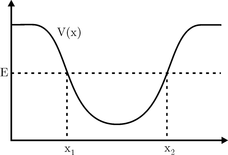
Schrödinger equation reads

\[ \frac{\mathrm{d}^2\Psi}{dz^2} - \frac{2m}{{\hbar}^2}\big[ E-V(z)\big]\Psi = 0 \]

Imagine there is an potential well between \(z_1\) and \(z_2\) shown in Figure 3.6: what are the allowable energy state?

In this case, \(k^2 = -\frac{2m}{{\hbar}^2}\big[ E-V(z)\big]\). Wave travelling to the right has positive \(k(z)\), while wave travelling to the left has negative \(k(z)\). Following the discussion of reflection coefficient,

\[ \begin{aligned} R = i e^{-2i \int_{0}^{z_2}k(z^\prime)dz^\prime} \\ R^\prime = i e^{+2i \int_{0}^{z_1}k(z^\prime)dz^\prime} \end{aligned} \]

For waves bouncing back and forth inside the well, we must have

\[ \begin{aligned} RR^\prime = 1 \\ \Rightarrow (-1)e^{-2i \int_{z_1}^{z_2}kdz^\prime} = 1 \\ \Rightarrow \int_{z_1}^{z_2}k(z^\prime)dz^\prime = \pi (n+\frac{1}{2}),\ n=0,1,2,3,... \end{aligned} \]

which is called the Bohr-Sommerfield quantization rule.

Another way to do this problem is by recognizing the Stokes and anti-Stokes lines in the complex z plane and match the solution in the whole domain. Figure needed!!! As the opposite in HW8.1%k2 .vs. z , Stokes line

\[ k^2 = -\frac{2m}{{\hbar}^2}\big[ E-V(z)\big] \equiv -p^2(z)(z-z_1)(z-z_2) \]

where for large z, we must choose a minus sign in front of \(p(z)\) for \(p(z)\) to be real and positive. So

\[ k = \pm i p(z)(z-z_1)^{1/2}(z-z_2)^{1/2} \]

Then for a single-value solution, pick

\[ \begin{aligned} -\pi\le\arg{(z-z_1)}<\pi \\ -\frac{\pi}{2}\le\arg{(z-z_2)}<\frac{3\pi}{2} \end{aligned} \]

For \(z\) on \(AS_1\),

\[ k(z) = \pm ip(z)|z-z_1|^{1/2} e^{i\frac{1}{2}\cdot0}\cdot |z-z_2|^{1/2}e^{i\frac{1}{2}\cdot \pi} = \pm i |k|e^{i\frac{1}{2}\pi} = \mp |k| \]

For a real and positive \(k\) (right-traveling wave), we must choose the lower sign \(+\), so

\[ k =- i p(z)(z-z_1)^{1/2}(z-z_2)^{1/2} \]

For \(z\) on \(S_1\), \[ k =- i p(z)|z-z_1|^{1/2}|z-z_2|^{1/2}= -i |k| \]

For \(z\) on \(S_4\),

\[ k =- i p(z)|z-z_1|^{1/2}e^{i\frac{1}{2}\pi}|z-z_2|^{1/2}e^{i\frac{1}{2}\pi}= i |k| \]

So

\[ k(z) = \begin{cases} -i|k| & z>z_2 \\ |k| & z_1<z<z_2 \\ i|k| & z<z_1 \end{cases} \tag{3.17}\]

On \(S_1\),

\[ \Psi_{E_{S_1}} \sim \frac{1}{\sqrt{k}}e^{\pm i \int_{z_2}^{z} kdz^\prime} = \frac{1}{\sqrt{k}}e^{-i\int_{z_2}^{z}kdz^\prime} \]

such that this is sub-dominant on \(S_1\) (\(k=-i|k|\)).

Crossing \(S_2\) into region I, we have

\[ \Psi_I \sim \frac{1}{\sqrt{k}}\Big\{ \underbrace{e^{-i\int_{z_2}^z kdz^\prime}}_{\text{dominant on }S_2} + i\underbrace{e^{+i\int_{z_2}^z kdz^\prime}}_{\text{subdominant on }S_2} \Big\} \tag{3.18}\]

On \(S_4\),

\[ \Psi_{S_4}\sim \frac{1}{\sqrt{k}}e^{\pm i \int_{z_1}^z kdz^\prime} \sim \frac{1}{\sqrt{k}}e^{-i\int_{z_1}^z kdz^\prime}, \]

where minus sign is chosen s.t. it is subdominant on \(S_4\).

Crossing \(S_3\) into region I in the clockwise direction, we have

\[ \begin{aligned} \Psi_I &\sim \Big\{ \underbrace{e^{-i\int_{z_1}^z kdz^\prime}}_{\text{dominant on }S_3} - i\underbrace{e^{+i\int_{z_1}^z kdz^\prime}}_{\text{subdominant on }S_3} \Big\} \\ &= \frac{1}{\sqrt{k}}\Big\{ e^{-i\int_{z_2}^z kdz^\prime}\cdot e^{-i\int_{z_1}^{z_2}kdz^\prime} - ie^{i\int_{z_2}^z kdz^\prime}\cdot e^{i\int_{z_1}^{z_2}kdz^\prime} \Big\} \end{aligned} \tag{3.19}\]

Because the solution is analytic, Equation 3.18 and Equation 3.19 should be equal, therefore

\[ \begin{aligned} &\frac{1}{e^{-i\int_{z_1}^{z_2}kdz^\prime}} = \frac{i}{-ie^{i\int_{z_1}^{z_2}kdz^\prime}} \\ \Rightarrow& e^{2i\int_{z_1}^{z_2}kdz^\prime} = -1 = e^{i(\pi+2n\pi)},\quad n=0,1,2,3,... \\ \Rightarrow& \int_{z_1}^{z_2}kdz^\prime = (\frac{1}{2}+n)\pi,\quad n=0,1,2,3,... \end{aligned} \]

Ex.4 Tunneling Problem

Instead of a potential well, now we consider another classical tunneling problem, where \(E>V\) if \(z_1<z<z_2\).

\[ k^2(z) = \pm p^2(z)(z-z_1)(z-z_2) = p^2(z)(z-z_1)(z-z_2) \]

where the plus sign is chosen s.t. \(p(z)\) is real and positive for all real z, and then

\[ k = p(z)(z-z_1)^{1/2}(z-z_2)^{1/2} \]

Define arguments as follows

\[ 0\le \arg{z-z_2} < 2\pi,\quad -\pi<\arg{z-z_1} \le \pi \]

to remove the ambiguity in the branch in the expression of \(k\).

Since \(z=z_1\), \(z=z_2\) are simple turning points (with different slope in linear approximation), the Stokes and anti-Stokes lines are shown in Figure needed!!!

The branch cut defined as above give the following values of \(k\) on the real \(z\) axis:

\[ k(z) = \begin{cases} |k| & z>z_2 \\ i|k| & z_1<z<z_2 \\ -|k| & z<z_1 \end{cases} \tag{3.20}\]

On \(AS_1\), the solution

\[ E\sim \frac{1}{\sqrt{k}}e^{-i\omega t+i \int_{z_2}^z kdz^\prime} \tag{3.21}\]

represents the outgoing wave propagating to \(z=\infty\).

On \(S_2\), solution Equation 3.21 behaves like \(E\sim e^{\int_b^z |k|dz^\prime}\) which is dominant on \(S_2\) with respect to \(z=z_2\). Thus, on \(S_1\), it is subdominant.

On crossing \(S_1\) from \(AS_1\), solution Equation 3.21 remains valid. In fact, it is valid in the region bounded by \(S_1\), \(S_2\) and \(S_3\). Note that it is subdominant on \(S_2\) with respect to \(z=z_1\) (because we just showed that it is dominant on \(S_2\) with respect to \(z=z_2\)). Thus, we rewrite the solution as

\[ E\sim \frac{1}{\sqrt{k}}e^{-i\omega t + i\int_{z_2}^{z_1} kdz^\prime}\cdot \underbrace{e^{i\int_{z_1}^z kdz^\prime}}_{\text{subdominant on }\ S_2 w.r.t\ z=a} \]

which becomes dominant on \(S_3\). Upon crossing \(S_3\), this solution becomes

\[ E\sim \frac{1}{\sqrt{k}}e^{-i\omega t + i\int_{z_2}^{z_1} kdz^\prime} \big[ \underbrace{e^{i\int_{z_1}^z kdz^\prime}}_{\text{dominant on }S_3} + \underbrace{ie^{-i\int_{z_1}^z kdz^\prime}}_{\text{subdominant on }S_3} \big] \]

where we pick up the Stokes constant \(i\) and the subdominant solution, represented by the last term of the solution.

Now, this is the solution on \(AS_4\) (\(z<z_1\)). Referring to Equation 3.20, we see that the first term of the solution represents the reflected wave, and the second term the incident wave from \(z=-\infty\). Since the incident wave and reflected wave have equal amplitude, we have

\[ |R|^2 = 1 \]

The transmitted wave has unit amplitude (see Eq.(\(\ref{eq-tunnel_AS1}\))). The incident wave has amplitude \(e^{i\int_a^b kdz^\prime}(i)\). Thus,

\[ |T|^2 = \frac{1}{\big| e^{i\int_{z_1}^{z_2} kdz^\prime}(i) \big|^2} = \frac{1}{\big| e^{i\int_{z_1}^{z_2} i|k|dz^\prime}(i) \big|^2} = e^{-2\int_{z_1}^{z_2} |k|dz} \]

where \(z_1,z_2\) are far apart, i.e. \(|T|^2\) is exponentially small.

Note: \(|R|\) and \(|T|\) above are not valid if \(z_1,z_2\) are close to each other. The correct transmission coefficient, for general valies of \(z_1,z_2\) is

\[ |T|^2 = \frac{e^{-2\int_{z_1}^{z_2} |k|dz}}{1+e^{-2\int_{z_1}^{z_2} |k|dz}} \]

and the reflection coefficient is

\[ |R|^2 = 1- |T|^2 \]

Ex.5 Two waves: one is launched from \(z=+\infty\), incident onto a resonant layer at \(z=a (a>0)\), and the other launched from \(z=-\infty\), incident onto a absorption layer at \(z=0\), with the model equation

\[ \frac{\mathrm{d}^2 E(z)}{dz} + {k_0}^2 \Big( \frac{z}{z-a}\Big) E(z) = 0 \]

This looks like a similar case for ECRH.

\[ k^2(z) = {k_0}^2 \Big( \frac{z}{z-a}\Big) \Rightarrow k(z) = k_0 z^{1/2}(z-a)^{-1/2} \]

where \(k_0\) is real and positive.

Define arguments as follows

\[ -\frac{3\pi}{2}\le \arg{z} < \frac{\pi}{2},\quad -\frac{3\pi}{2}<\arg{z-a} \le \frac{\pi}{2} \]

to remove the ambiguity in the branch in the expression of \(k\).

For \(z\) on \(AS_1\),

\[ k = k_0 |z|^{1/2}e^{-\frac{1}{2}0}|z-a|^{-1/2}e^{i\frac{1}{2}0} = |k| \]

For \(z\) on \(S_1\),

\[ k = k_0 |z|^{1/2}e^{-\frac{1}{2}0}|z-a|^{-1/2}e^{i\frac{1}{2}\pi} = i|k| \]

For \(z\) on \(AS_2\),

\[ k = k_0 |z|^{1/2}e^{i\frac{1}{2}(-\pi)}|z-a|^{-1/2}e^{i\frac{-1}{2}(-\pi)} = |k| \]

Then the branch cut defined as above give the following values of \(k\) on the real \(z\) axis:

\[ k(z) = \begin{cases} |k| & z>a \\ i|k| & 0<z<a \\ |k| & z<0 \end{cases} \tag{3.22}\]

For wave launched from large magnetic field side \(z=+\infty\) going to \(z=-\infty\) on \(AS_3\), the solution on \(AS_3\) is (Note that even though \(z\) is negative, it is the upper limit of the integral and k is positive. It took me a long time to get the right sign here for a left propagating wave.)

\[ E\sim \frac{1}{\sqrt{k}}e^{-i\omega t- i \int_0^z kdz^\prime} \] This solution behaves like

\[ E\sim \frac{1}{\sqrt{k}} e^{-i\omega t- i \int_0^z i|k|dz^\prime} \sim \frac{1}{\sqrt{k}} e^{-i\omega t + \int_0^z |k|dz^\prime} \tag{3.23}\]

on \(S_1\). Thus, it is dominant on \(S_1\) with respect to \(z=0\); it is subdominant on the neighboring Stokes line \(S_2\). Thus solution Equation 3.23 remains valid upon crosing Stokes line \(S_2\). It is the solution in region I, bounded by \(S_1\) and \(S_2\). Since it is dominant on \(S_1\) with respect to \(z=0\), it is subdominant on \(S_1\) with respect to \(z=a\). So we can write it as

\[ E \sim \frac{1}{\sqrt{k}}e^{-i\omega t - i\int_0^a kdz^\prime}\cdot \underbrace{e^{-i\int_a^z kdz^\prime}}_{\text{subdominant on }\ S_1\ w.r.t.\ z=a} \]

which is also the incident wave from \(z=0\). This is the solution in region I as well as on \(AS_1\) (\(k=|k|\)). So it is the incident wave solution from \(z=\infty\). The reflection coefficient must be 0!

The transmisson coefficient is then

\[ \begin{aligned} |T|^2 &= \Big| \frac{E(z=-\infty)}{E(z=\infty)} \Big|^2 = \frac{1}{|e^{-i\int_0^a kdz}|^2} \notag \\ &= e^{-2\int_0^a |k| dz} = e^{-2\int_0^a k_0 \sqrt{\frac{z}{a-z}}dz} \end{aligned} \]

Let \(z=a\sin^2\theta\), we can finally have

\[ |T|^2 = e^{-k_0 a\pi} \]

The fraction of power absorbed by resonance is

\[ 1-|R|^2 - |T|^2 = 1-e^{-k_0 a \pi} \]

Note: these expressions of \(|T|^2, \ |R|^2\) are valid even if \(a\) is small.

For wave launched from low magnetic field side \(z=-\infty\),

\[ E_{AS_1} \sim\frac{1}{\sqrt{k}}e^{-i\omega t + i \int_a^z kdz^\prime} \]

On \(S_1\), a subdominant (decaying) solution with respect to \(z=0\) is

\[ E_{S_1}\sim \frac{1}{\sqrt{k}}e^{-i\omega t+i\int_0^z i|k|dz^\prime} \]

In regions I bounded by \(S_1,\ S_2\) and \(AS_1\),

\[ E_I \sim E_{S_1}\frac{1}{\sqrt{k}}e^{i\int_a^0 kdz^\prime}\cdot e^{i\int_0^z kdz^\prime} \]

\(E_{S_1}\) is dominant on \(S_1\) with respect to \(z=a\), but is subdominant on \(S_1\) with respect to \(z=0\).

Crossing \(S_2\) into \(AS_2\),

\[ E_{AS_2}\sim \frac{1}{\sqrt{k}}e^{-i\omega t}\cdot e^{i\int_a^0 kdz^\prime}\Big[ \underbrace{e^{i\int_0^z kdz^\prime}}_{\text{dominant on }S_3} - i \underbrace{e^{-i\int_0^z kdz^\prime}}_{\text{subdominant on }S_3} \Big], \]

where the first term represents the reflected wave, and the second term represents the incident wave.

The transmission coefficient is

\[ \begin{aligned} T &= \Big| \frac{E(z=\infty)}{E(z=-\infty)} \Big| \\ &=\Big|\frac{\sqrt{k(-\infty)}}{\sqrt{k(\infty)}} \Big| \Big| \frac{e^{i\int_a^\infty kdz}}{e^{i\int_a^0 kdz}\cdot e^{i\int_0^{-\infty} kdz}} \Big| \\ &=\frac{1}{\big| e^{i\int_a^0 i|k|dz} \big|} = e^{-\int_0^a |k|dz} \end{aligned} \]

Then the transmission coefficient in power is

\[ T^2 = e^{-2\int_0^a k \sqrt{|\frac{z}{z-a}|}dz^\prime } = e^{-k_0 a \pi} \]

where the last equivalence requires some transformation tricks. If \(a\sim\lambda, k_0 = 2\pi/\lambda\), the transmitted power fraction is on the order of \(e^{-20}\sim 10^{-9}\).

The reflection coefficient is zero and that the transmission coefficient (in power) is \(T=e^{-k_0 a\pi}\). Thus, the fraction \(1-T\) of the incident power is absorbed by that resonant layer.

3.11.5 “Exact” WKBJ Solution

• Shielding or tunneling

If you have a high density region between \(x_1\) and \(x_2\),

\[ k^2(x) = \frac{\omega^2}{c^2}\big[ 1-\frac{{\omega_p}^2(x)}{\omega^2}\big] \]

The transmission coefficient in power is

\[ |T|^2 = \frac{e^{-2\int_{x_1}^{x_2}|k|\mathrm{d}x}}{1+e^{-2\int_{x_1}^{x_2}|k|\mathrm{d}x}} \]

and the reflection coefficient in power is

\[ |R|^2 = \frac{1}{1+e^{-2\int_{x_1}^{x_2}|k|\mathrm{d}x}} \]

Note:

• \(|R|^2+|T|^2 = 1\)

• When \(x_1=x_2\), i.e. \(\omega^2 = {\omega_p}^2(\text{peak})\), \(|R|^2=|T|^2=\frac{1}{2}\).

• ECRH

\[ \frac{\mathrm{d}^2E}{dz^2} + {k_0}^2\Big( \frac{z}{z-a}\Big)E = 0 \]

where

\[ k^2(z) = {k_0}^2\Big( \frac{z}{z-a}\Big) \]

1. Incident wave from \(z=-\infty\) (from low \(B_0\) side)

\[ \begin{aligned} |R| &= 1 - e^{-\pi k_0 a} \\ |T| &= e^{-\frac{1}{2}\pi k_0 a} \\ |R|^2 + |T|^2 &= 1-e^{-\pi k_0 a} + e^{-2\pi k_0 a} <1 \end{aligned} \]

2. Incident wave from \(z=\infty\)

\[ \begin{aligned} |R| &= 0 \\ |T| &= e^{-\pi k_0 a/2} \\ |R|^2 + |T|^2 &= e^{-\pi k_0 a} < 1 \end{aligned} \]

which means almost perfect absorption at \(z=a\).

Note: These formulas are valid even if \(a\rightarrow0\), in which limit \(|R|\rightarrow 0,\ |T|\rightarrow 1\), for both (I) and (II), as expected from the model equation.

Singularity in refractive index \(n\) can lead to absorption, even without collision.

3.12 Normalization

In physics we frequently have to deal with unit conversions. A solid understanding of the unit system and normalization methods paves the path for understanding the scales behind systems.

3.13 Theoretical Mechanics

Newtonian mechanics is great, but theoretical mechanics is marvellous. It does not tell you anything new, but let you think of the same thing from a different prospective. Theoretical mechanics takes advantage of a system’s constraints to solve problems. The constraints limit the degrees of freedom the system can have, and can be used to reduce the number of coordinates needed to solve for the motion. The formalism is well suited to arbitrary choices of coordinates, known in the context as generalized coordinates. The kinetic and potential energies of the system are expressed using these generalized coordinates or momenta, and the equations of motion can be readily set up, thus analytical mechanics allows numerous mechanical problems to be solved with greater efficiency than fully vectorial methods. It does not always work for non-conservative forces or dissipative forces like friction, in which case one may revert to Newtonian mechanics.

3.13.1 Generalized Coordinates

In Newtonian mechanics, one customarily uses all three Cartesian coordinates, or other 3D coordinate system, to refer to a body’s position during its motion. In physical systems, however, some structure or other system usually constrains the body’s motion from taking certain directions and pathways. So a full set of Cartesian coordinates is often unneeded, as the constraints determine the evolving relations among the coordinates, which relations can be modeled by equations corresponding to the constraints. In the Lagrangian and Hamiltonian formalisms, the constraints are incorporated into the motion’s geometry, reducing the number of coordinates to the minimum needed to model the motion. These are known as generalized coordinates, denoted \(q_i\, (i = 1, 2, 3...)\).

3.13.2 D’Alembert’s Principle

This principle is the analogy of Newton’s second law in theoretical mechanics. It states that infinitesimal virtual work done by a force across reversible displacements is zero, which is the work done by a force consistent with ideal constraints of the system. The idea of a constraint is useful — since this limits what the system can do, and can provide steps to solving for the motion of the system. The equation for D’Alembert’s principle is: \[ \delta W = \mathbf{Q}\cdot \mathrm{d}\mathbf{q} = 0 \] where \[ \mathbf{Q} = (Q_1, Q_2, ..., Q_N) \] are the generalized forces (script Q instead of ordinary Q is used here to prevent conflict with canonical transformations below) and \(\mathbf{q}\) are the generalized coordinates. This leads to the generalized form of Newton’s laws in the language of theoretical mechanics: \[ \mathbf{Q} = \frac{\mathrm{d}}{\mathrm{d}t}\Big( \frac{\partial T}{\partial\dot{\mathbf{q}}} \Big) - \frac{\partial T}{\partial\mathbf{q}} \] where T is the total kinetic energy of the system, and the notation \[ \frac{\partial}{\partial\mathbf{q}} = \Big( \frac{\partial}{\partial q_1},\frac{\partial}{\partial q_2}, ..., \frac{\partial}{\partial q_N} \Big) \]

3.13.3 Lagrangian Mechanics

Lagrangian and Euler–Lagrange equations

The introduction of generalized coordinates and the fundamental Lagrangian function: \[ L(\mathbf{q},\dot{\mathbf{q}},t) = T(\mathbf{q},\dot{\mathbf{q}},t) - V(\mathbf{q},\dot{\mathbf{q}},t) \] where \(T\) is the total kinetic energy and \(V\) is the total potential energy of the entire system, then either following the calculus of variations or using the above formula — lead to the Euler-Lagrange equations; \[ \frac{\mathrm{d}}{\mathrm{d}t}\Big( \frac{\partial L}{\partial\dot{\mathbf{q}}} \Big) = \frac{\partial L}{\partial\mathbf{q}} \] which are a set of N second-order ordinary differential equations, one for each \(q_i(t)\). This formulation identifies the actual path followed by the motion as a selection of the path over which the time integral of kinetic energy is least, assuming the total energy to be fixed, and imposing no conditions on the time of transit.

3.13.4 Hamiltonian Mechanics

Hamiltonian and Hamilton’s equations

The Legendre transformation of the Lagrangian replaces the generalized coordinates and velocities \((\mathbf{q}, \dot{\mathbf{q}})\) with \((\mathbf{q}, \mathbf{p})\); the generalized coordinates and the generalized momenta conjugate to the generalized coordinates: \[ \mathbf{p} = \frac{\partial L}{\partial\dot{\mathbf{q}}} = \Big(\frac{\partial L}{\partial\dot{q}_1},\frac{\partial L}{\partial\dot{q}_2},,...,\frac{\partial L}{\partial\dot{q}_N} \Big) = (p_1, p_2, ..., p_N) \] and introduces the Hamiltonian (which is in terms of generalized coordinates and momenta): \[ H(\mathbf{q},\mathbf{p},t) = \mathbf{p}\cdot\dot{\mathbf{q}} - L(\mathbf{q},\dot{\mathbf{q}},t) \]

This leads to the Hamilton’s equations: \[ \dot{\mathbf{p}} = -\frac{\partial H}{\partial\mathbf{q}},\quad\dot{\mathbf{q}} = \frac{\partial H}{\partial \mathbf{p}} \]

which are now a set of 2N first-order ordinary differential equations, one for each \(q_i(t)\) and \(p_i(t)\). Another result from the Legendre transformation relates the time derivatives of the Lagrangian and Hamiltonian: \[ \frac{dH}{\mathrm{d}t} = -\frac{\partial L}{\partial t} \] which is often considered one of Hamilton’s equations of motion additionally to the others. The generalized momenta can be written in terms of the generalized forces in the same way as Newton’s second law: \[ \dot{\mathbf{p}} = \mathbf{Q} \]

One interesting application of the Hamilton’s equation in plasma physics is the prove of Vlasov equation (See Giulia’s notes) \[ \frac{df(\mathbf{q},\mathbf{p},t)}{\mathrm{d}t} = 0 \]

You may also find the application in deriving the gyrokinetic equations.

3.13.5 Hamilton-Lagrange formalism vs. Lorentz equation

Two mathematically equivalent formalisms describe charged particle dynamics, namely

1. the Lorentz equation \[ m\frac{\mathrm{d}\mathbf{v}}{\mathrm{d}t} = q(\mathbf{E} + \mathbf{v}\times\mathbf{B}) \]

2. Hamiltonian-Lagrangian dynamics.

The two formalisms are complementary: the Lorentz equation is intuitive and suitable for approximate methods, whereas the more abstract Hamiltonian-Lagrangian formalism exploits time and space symmetries. A brief review of the Hamiltonian-Lagrangian formalism follows, emphasizing aspects relevant to dynamics of charged particles.

The starting point is to postulate the existence of a function \(L\), called the Lagrangian, which:

1. contains all information about the particle dynamics for a given situation;
2. depends only on generalized coordinates \(Q_i(t),\dot{Q}_i(t)\) appropriate to the problem;
3. possibly has an explicit dependence on time \(t\).

If such a function \(L(Q_i(t), \dot{Q}_i(t), t)\) exists, then information on particle dynamics is retrieved by manipulation of the action integral \[ S = \int_{t_1}^{t_2}L(Q_i(t), \dot{Q}_i(t), t) \mathrm{d}t \]

This manipulation is based on d’Alembert’s principle of least action. According to this principle, one considers the infinity of possible trajectories a particle could follow to get from its initial position \(Q_{i}(t_1)\) to its final position \(Q_i(t_2)\), and postulates that the trajectory actually followed is the one that results in the lowest value of \(S\). Thus, the value of \(S\) must be minimized (note that \(S\) here is action, and not entropy). Minimizing \(S\) does not give the actual trajectory directly, but rather gives equations of motion, which can be solved to give the actual trajectory.

Minimizing \(S\) is accomplished by considering an arbitrary nearby alternative trajectory \(Q_i(t)+\delta Q_i(t)\) having the same beginning and end points as the actual trajectory, i.e., \(\delta Q_i(t_1)=Q_i(t_2)=0\). In order to make the variational argument more precise, \(\delta Q_i\) is expressed as \[ \delta Q_i(t) = \epsilon \eta_i(t) \] where \(\epsilon\) is an arbitrarily adjustable scalar assumed to be small so that \(\epsilon^2 < \epsilon\) and \(\eta_i(t)\) is a function of \(t\) that vanishes when \(t=t_1\) or \(t=t_2\) but is otherwise arbitrary. Calculating \(\delta S\) to second order in \(\epsilon\) gives \[ \begin{aligned} \delta S &= \int_{t_1}^{t_2}L(Q_i+\delta Q_i, \dot{Q}_i + \delta\dot{Q}_i, t) \mathrm{d}t - \int_{t_1}^{t_2}L(Q_i(t), \dot{Q}_i(t), t) \mathrm{d}t \\ &= \int_{t_1}^{t_2}L(Q_i+\epsilon\eta_i, \dot{Q}_i + \epsilon \dot{\eta}_i, t) \mathrm{d}t - \int_{t_1}^{t_2}L(Q_i(t), \dot{Q}_i(t), t) \mathrm{d}t \\ &= \int_{t_1}^{t_2} \left( \epsilon\eta_i\frac{\partial L}{\partial Q_i} + \frac{(\epsilon \eta_i)^2}{2}\frac{\partial^2 L}{\partial Q_i^2} + \epsilon \dot{\eta}_i\frac{\partial L}{\partial\dot{Q}_i} + \frac{(\epsilon\dot{\eta}_i)^2}{2}\frac{\partial^2 L}{\partial\dot{Q}_i^2} \right)\mathrm{d}t \end{aligned} \]

Suppose the trajectory \(Q_i(t)\) is the one that minimizes \(S\). Any other trajectory must lead to a higher value of \(S\) and so \(\delta S\) must be positive for any finite value of \(\epsilon\). If \(\epsilon\) is chosen to be sufficiently small, then the absolute values of the terms of order \(\epsilon^2\) above will be smaller than the absolute values of the terms linear in \(\epsilon\). The sign of \(\epsilon\) could then be chosen to make \(\delta S\) nagative, but this would violate the requirement that \(\delta S\) must be positive. The only way out of this dilemma is to insist that the sum of the terms linear in \(\epsilon\) vanishes so \(\delta S\sim \epsilon^2\) and is therefore always positive as required. Insisting that the sum of terms linera in \(\epsilon\) vanishes implies \[ 0 = \int_{t_1}^{t_2} \left( \eta_i\frac{\partial L}{\partial Q_i} + \dot{\eta}_i\frac{\partial L}{\partial\dot{Q}_i} \right)\mathrm{d}t \]

Using \(\dot{\eta}_i = \mathrm{d}\eta_i/\mathrm{d}t\) the above expression may be integrated by parts to obtain \[ \begin{aligned} 0 &= \int_{t_1}^{t_2} \left( \eta_i\frac{\partial L}{\partial Q_i} + \dot{\eta}_i\frac{\partial L}{\partial\dot{Q}_i} \right)\mathrm{d}t \\ &= \left[ \eta_i\frac{\partial L}{\partial \dot{Q}_i} \right]_{t_1}^{t_2} + \int_{t_1}^{t_2}\left[ \eta_i\frac{\partial L}{\partial Q_i} - \eta_i\frac{\mathrm{d}}{\mathrm{d}t}\left( \frac{\partial L}{\partial \dot{Q}_i} \right) \right]\mathrm{d}t \end{aligned} \]

Since \(\eta_i(t_{1,2})=0\), the integrated term vanishes and since \(\eta_i\) was an arbitrary function of \(t\), the coefficient of i in the integrand must vanish, yielding Lagrange’s equation \[ \frac{\mathrm{d}P_i}{\mathrm{d}t} = \frac{\partial L}{\partial Q_i} \tag{3.24}\] where the canonical momentum \(P_i\) is defined as \[ P_i \equiv \frac{\partial L}{\partial\dot{Q}_i} \tag{3.25}\]

Lagrange’s equation shows that if \(L\) does not depend on a particular generalized coordinate \(Q_j\), then \(\mathrm{d}P_j/\mathrm{d}t=0\), in which case the canonical momentum \(P_j\) is a constant of motion; the coordinate \(Q_j\) is called a cyclic or ignorable coordinate. This is a very powerful and profound result. Saying that the Lagrangian function does not depend on a coordinate is equivalent to saying that the system is symmetric in that coordinate or translationally invariant with respect to that coordinate. The quantities \(P_j\) and \(Q_j\) are called conjugate and action has the dimensions of the product of these quantities.

Hamilton extended this formalism by introducing a new function related to the Lagrangian. This new function, called the Hamiltonian, provides further useful information and is defined as \[ H \equiv \left( \sum_i P_i \dot{Q}_i \right) - L \tag{3.26}\]

Partial derivative of \(H\) with respect to \(P_i\) and to \(Q_i\) give Hamilton’s equations \[ \dot{Q}_i = \frac{\partial H}{\partial P_i},\quad \dot{P}_i = -\frac{\partial H}{\partial Q_i} \] which are equations of motion having a close relation to phase-space concepts. The time derivative of the Hamiltonian is \[ \frac{\mathrm{d}H}{\mathrm{d}t} = \sum_i \frac{\mathrm{d}P_i}{\mathrm{d}t}\dot{Q}_i + \sum_i P_i\frac{\mathrm{d}\dot{Q}_i}{\mathrm{d}t} - \left( \sum_i\frac{\partial L}{\partial Q_i}\dot{Q}_i + \sum_i\frac{\partial L}{\partial\dot{Q}_i}\frac{\mathrm{d}\dot{Q}_i}{\mathrm{d}t} + \frac{\partial L}{\partial t} \right) = -\frac{\partial L}{\partial t} \tag{3.27}\]

This shows that if Ldoes not explicitly depend on time, the Hamiltonian \(H\) is a constant of the motion. As will be shown later, \(H\) corresponds to the energy of the system, so if \(\partial L/\partial t=0\), the energy is a constant of the motion. Thus, energy is conjugate to time in analogy to canonical momentum being conjugate to position (note that energy \(\times\) time also has the units of action). If the Lagrangian does not explicitly depend on time, then the system can be thought of as being “symmetric” with respect to time, or “translationally” invariant with respect to time.

The Lagrangian for a charged particle in an electromagnetic field is \[ L = \frac{mv^2}{2} + q\mathbf{v}\cdot\mathbf{A}(\mathbf{x},t) - q\phi(\mathbf{x},t) \tag{3.28}\]

The validity of Equation 3.28 will now be established by showing that it generates the Lorentz equation when inserted into Lagrange’s equation. Since no symmetry is assumed, there is no reason to use any special coordinate system and so ordinary Cartesian coordinates will be used as the canonical coordinates, in which case Equation 3.25 gives the canonical momentum as \[ \mathbf{P} = m\mathbf{v} + q\mathbf{A}(\mathbf{x},t) \]

The left-hand side of Equation 3.24 becomes \[ \frac{\mathrm{d}\mathbf{P}}{\mathrm{d}t} = m\frac{\mathrm{d}\mathbf{v}}{\mathrm{d}t} + q\left( \frac{\partial\mathbf{A}}{\partial t} + \mathbf{v}\cdot\nabla\mathbf{A} \right) \] while the right-hand side of Equation 3.24 becomes \[ \begin{aligned} \frac{\partial L}{\partial\mathbf{x}} &= q\nabla(\mathbf{v}\cdot\mathbf{A}) - q\nabla\phi = q(\mathbf{v}\cdot\nabla\mathbf{A} + \mathbf{v}\times\nabla\times\mathbf{A}) - q\nabla\phi \\ &= q(\mathbf{v}\cdot\nabla\mathbf{A} + \mathbf{v}\times\mathbf{B}) - q\nabla\phi \end{aligned} \]

Equating the above two expressions gives the Lorentz equation, where the electric field is defined as \(\mathbf{E}=-\partial\mathbf{A}/\partial t - \nabla\phi\) in accordance with Faraday’s law. This proves that Equation 3.28 is mathematically equivalent to the Lorentz equation when used with the principle of least action.

The Hamiltonian associated with this Lagrangian is, in Cartesian coordinates, \[ \begin{aligned} H &= \mathbf{P}\cdot\mathbf{v} - L = \frac{mv^2}{2} + q\phi \\ &= \frac{\left(\mathbf{P} - q\mathbf{A}(\mathbf{x},t)\right)^2}{2m} + q\phi(\mathbf{x},t) \end{aligned} \tag{3.29}\] where the last line is the form more suitable for use with Hamilton’s equations, i.e., \(H=H(\mathbf{x},\mathbf{P},t)\). Equation 3.29 also shows that \(H\) is, as promised, the particle energy. If generalized coordinates are used, the energy can be written in a general form as \(E=H(Q,P,t)\). Equation 3.27 showed that even though both \(Q\) and \(P\) depend on time, the energy depends on time only if \(H\) explicitly depends on time. Thus, in a situation where \(H\) does not explicitly depend on time, the energy would have the form \(E=H(Q(t),P(t)) = \mathrm{const}\).

It is important to realize that both canonical momentum and energy depend on the reference frame. For example, a bullet fired in an airplane in the direction opposite to the airplane motion, and with a speed equal to the airplane’s speed, has a large energy as measured in the airplane frame, but zero energy as measured by an observer on the ground. A more subtle example (of importance to later analysis of waves and Landau damping) occurs when \(\mathbf{A}\) and/or \(\phi\) has a wave-like dependence, e.g., \(\phi(\mathbf{x},t)=\phi(\mathbf{x}-\mathbf{v}_{\mathrm{ph}}t)\), where \(\mathbf{v}_{\mathrm{ph}}\) is the wave phase velocity. This potential is time-dependent in the lab frame and so the associated Lagrangian has an explicit dependence on time in the lab frame, which implies that energy is not a constant of the motion in the lab frame. In contrast, \(\phi\) is time-independent in the wave frame and so the energy is a constant of the motion in the wave frame. Existence of a constant of the motion reduces the complexity of the system of equations and typically makes it possible to integrate at least one equation in closed form. Thus, it is advantageous to analyze the system in the frame having the most constants of the motion.

3.14 Wavelet Analysis

Wavelet Transform (WT) decomposes a function into a set of wavelets. A Wavelet is a wave-like oscillation that is localized in time. Two basic properties of a wavelet are scale and location.

Wavelet is a predecessor of Fourier Tranform (FT), which provides better results when dealing with changing background. It is the de-facto method for modern wave analysis. The key advantages of WT compared with FT are:

• Fewer “hard” parameters to tune in WT. For example, if you want to make a spectrogram with FT, you need to specify the size of local DFTs. In WT you do not need to worry about this; instead the validity of the result can be shown by the cone of influence. In a sense, FT makes immediate conversion from time to frequency domain, while WT let you choose the intermediate steps you wish for.
• Flexible forms of wavelets to choose from. In practice, if you have any prior knowledge to the signal you want to identify, you can find for an appropriate wavelet that is close to that shape, which gives better fitting compared to the sinuisoidal functions in FT.

Check the notes from my blog and the references therein.

Budden, Kenneth George. 1961. Radio Waves in the Ionosphere. Radio Waves in the Ionosphere.