30 Hybrid Methods
The hybrid model is valid for low-frequency physics with \(\omega\sim\Omega_i\) and \(kr_{Li}\sim 1\) (wavelength \(\lambda\sim 6r_{Li}\)), where \(\omega\) is the wave frequency, \(k\) is the wave number, \(\Omega_i\) is the ion gyrofrequency, and \(r_{Li}\) is the ion Larmor radius. For this range of wave frequency and wavelength, the ion kinetic physics in the near-Earth instabilities are resolved with grid sizes \(\sim r_{Li}\) or ion inertial length \(d_i\). The finite ion gyroradius effects are resolved with particle time steps \(\Delta t\) much smaller than the gyroperiod.
A typical time step in a global hybrid magnetosphere model is \(0.05\,\Omega_0^{-1}\), where \(\Omega_0\) is the upstream (solar wind) ion gyrofrequency. For IMF \(B_0\sim10\,\text{nT}\), \(\Omega_0 \sim 1\,\text{rad/s}\), which corresponds to \(f_0\sim 1/2\pi\,\text{s}^{-1}\). Based on in-situ observations, the typical ion inertial length in the tail is \(\sim 0.2\,\text{R}_\text{E}\), but smaller near the dayside magnetopause. Therefore usually discrete grid size \(\Delta x = 0.1\,d_i\) is barely enough to resolve tail ion kinetic dynamics but not dayside kinetic structures.
30.1 Classical Hybrid Model
Define the electric charge density \(\rho\) and current density \(\mathbf{J}\) as \[ \rho = \sum_s q_s n_s - en_e \]
\[ \mathbf{J} = \sum_s q_s n_s \mathbf{u}_s - e n_e \mathbf{u}_e \] where \(q_s, n_s, \mathbf{U}_s\) are the charge, number density and bulk velocity of ion species s calculated by taking moments of the distribution function \[ n_s = \int \mathrm{d}^3 v f_s(\mathbf{r}_s,\mathbf{v}_s,t) \] \[ \mathbf{u}_s = \frac{1}{n_s}\int \mathrm{d}^3 v \mathbf{v}_s f_s(\mathbf{r}_s,\mathbf{v}_s,t) \] or in the corresponding discrete forms where the distribution function is represented as a group of macro-particles with a specific shape function. In this way it behaves more like a particle cloud.
The crucial assumption in the hybrid model is the quasi-neutrality, that is, the electrons move fast enough to cancel any charge-density fluctuations and \(\rho=0\) is always satisfied. By assuming quasi-neutrality, we can
- avoid solving the conservation equations for electrons
- avoid solving the Maxwell’s equations entirely and instead use the generalized Ohm’s law instead
The electron density thus can be written by using ion densities \(n_e \approx n_i \equiv \sum_s q_s n_s /e\). In addition, the electron bulk velocity may also be eliminated using Ampère’s law \[ \mathbf{J} = \mu_0^{-1}\nabla\times\mathbf{B} \tag{30.1}\] and the relation \[ \mathbf{u}_e = \mathbf{u}_i - \mathbf{J}/n_e e \tag{30.2}\]
The basic equations used in the conventional PIC hybrid model first has a particle pusher for individual ions \[ \frac{\mathrm{d}\mathbf{x}_j}{\mathrm{d}t} = \mathbf{v}_j \]
\[ \frac{\mathrm{d}\mathbf{v}_j}{\mathrm{d}t} = \frac{q_j}{m_j}\big( \mathbf{E} + \mathbf{v}_j \times \mathbf{B} \big) \] where the subscript \(j\) and \(e\) indicate the indices for individual ions and the electron fluid and other notations are standard. The lowercase velocities are velocities for each macro-particle.
Alternatively, if we rely on a Vlasov system, we directly solve for the distribution function \(f(\mathbf{r}_s, \mathbf{v}_s, t)\) from the Vlasov equation \[ \frac{\partial f_s}{\partial t} + \mathbf{v}_s\frac{\partial f_s}{\partial \mathbf{r}_s} + \mathbf{a}_s\cdot \frac{\partial f_s}{\partial \mathbf{v}_s} = 0 \] where \[ \mathbf{a}_s = \frac{q_s}{m_s}(\mathbf{E}+\mathbf{v}_s\times\mathbf{B}) \]
The generalized Ohm’s law is used to determine the time evolution of the electric field, derived from the electron momentum equation assuming \(m_e \rightarrow 0\), \[ \mathbf{E} = - \mathbf{u}_i \times \mathbf{B} + \frac{1}{\mu_0 n_e e}(\nabla\times\mathbf{B})\times\mathbf{B} - \frac{1}{n_e e}\nabla\cdot\overleftrightarrow{P}_e + \mathbf{R}_{ei} \tag{30.3}\] where the current in the Hall term has already been replaced by the curvature of B. Note that the density has been written with electron number density, instead of ion density, to avoid the confusion for multiple ion species under the quasi-neutrality condition. The last term \(\mathbf{R}_{ei}\) can either represent collision/physical resistivity, or artificial resistivity/numerical diffusion. For electromagnetic problems, it can include resistive and hyper-resistive terms of the form \[ \mathbf{R}_{ei} = \eta \mathbf{J} + \eta_H\nabla^2\mathbf{J} \] where the resistivity \(\eta\) may be thought of as accounting in a simple way for electron-ion collisions, and the hyper-resistivity \(\eta_H\) may represent an electron viscosity and helps with numerical stability by damping grid-scale oscillations. In addition, \(\mathbf{R}_{ei}\) can also include contributions from explicit friction or other momentum exchange terms in the particle collision models.
The magnetic fields evolve according to Faraday’s law \[ \frac{\partial \mathbf{B}}{\partial t} = -\nabla\times\mathbf{E} \]
The Hall term supports Whistler waves, which usually place the strongest limit on the time step in hybrid PIC codes. The Courant–Friedrichs–Lewy (CFL) condition for Whistler waves on the time step is typically \(\Omega_{ci}\Delta t < (\Delta x/ d_i)^2/\pi\). Updating the magnetic field including the Hall term turns out to be a stiff problem, thus requires smaller time step sub-cycling in many practical cases. This is most useful when the grid resolution is very fine with \(\Delta x\ll d_i\).
Finally, by determining the electron pressure tensor by using an appropriate equation of state, the evolution of the system can be followed in time. For example, let \(\overleftrightarrow{P}_e = P_e \overleftrightarrow{I}\) where \(P_e\) is the isotropic scalar electron pressure. In the simplest form \[ P_e = n_e k_B T_e \] where \(n_e \approx n_i\) and \(T_e=T_i\). Note however in a plasma electron pressure is usually higher than ion temperature, so this is a very crude assumption. Another commonly used assumption is an adiabatic process \[ P_e = n_e^\gamma k_B T_e = n_0(n/n_0)^\gamma k_B T_{e0} \] where \(\gamma=5/3\) is the adiabatic index for a monatomic ideal gas.
For more complicated systems with gradients in the initial conditions, a separate electron energy evolution equation is required. This takes the form \[ \frac{\partial P_e}{\partial t} = -\gamma \nabla\cdot(P_e \mathbf{u}_e) + (\gamma-1)\mathbf{u}_e\cdot\nabla P_e + (\gamma-1)(-\nabla\cdot\mathbf{Q}_e + H_{ei}) \tag{30.4}\] where the electron bulk velocity is inferred from Equation 30.2, with the current from Equation 30.1. If used in place of a simple equation of state, Equation 30.4 is integrated in time within the same numerical loop as the magnetic field evolution. For many problems, the electron heat flux may be modeled with a heat conductivity \(\kappa\) as \[ \mathbf{Q_e} = -\kappa \nabla T_e \] where \(\kappa = \kappa_e + \kappa_0\), \(\kappa_e\) is given by a physical model and may depend on the local plasma conditions, and \(\kappa_0\) is a small (\(\kappa_0\sim 0.01 - 0.1 \kappa_e\) for models with a physical heat conductivity, or \(\kappa_0\sim 0.01 n_0 d_i V_A\) for magnetized simulations) constant numerical diffusion coefficient set separately for convenience that helps maintain numerical stability. Models for electron and ion energy exchange may be included through the term \(H_{ei}\), which can be captured by adding energy lost in each cell by ions in collisions models back to the local electron fluid cell. (???)
It is of course possible to incorporate the full electron pressure tensor effects to handle specially reconnection physics better.
A more complete review is given by (Winske et al. 2023) for the hybrid-kinetic model assuming massless electrons. The essential problem in all hybrid algorithms is how to calculate the electric field at the next time step.
30.1.1 Pros and Cons
Strengths:
- No approximations to ion physics.
- Valid for \(\omega/\Omega_i \sim kr_i \sim 1\).
- No issues for high-\(\beta\) regimes.
- Simple implementation of particle push that can be readily optimized.
- Removes stiffest electron scales. Neglecting the electron kinetic scales typically reduces the computing cost and memory requirements by a factor of \(\sqrt{m_i/m_e}\) (compared to what is used in full-PIC) for each spatial dimension and the time step may usually be increased by a similar factor.
Limitations:
- Need to resolve ion gyrofrequency.
- Stiff EMHD whistler waves \(\Delta t_{CFL}\sim \Delta x^2\).
- No electron Landau damping.
- Explicit time-stepping schemes can be complex.
- No existing method conserves momentum or energy.
30.1.2 Role of Electrons
The interpretation of “massless” electrons is tricky. If we think of the full particle model, and take the asymptotic behavior when \(m_e\to 0\), this does not explicitly lead to the hybrid equations. The reason is that
- The hybrid model completely eliminates the electron inertia term from the equations of motion. This is not just an approximation of small mass; it fundamentally changes the way electrons respond to fields.
- Hybrid models often (though not always) assume quasi-neutrality, where the electron and ion densities are nearly equal. This is a separate assumption from massless electrons.
- The way the electric and magnetic fields are calculated differs between the two models. The hybrid model typically solves for the electric field directly from a combination of the generalized Ohm’s law and Faraday’s law, whereas the full particle model would solve Maxwell’s equations fully. Again, combined with point 1, the way electrons respond to fields is completely different in the two models.
30.1.3 Minimum Resolution Limit
Interestingly, hybrid models set a lower bound on the simulation cell size \(\Delta L\) (often \(\Delta L \gtrsim 10 \delta_e\)) primarily to ensure the physical consistency of the “massless electron” approximation and to maintain numerical stability. In standard hybrid plasma models (kinetic ions, massless fluid electrons), resolving the electron inertial length \(\delta_e\) can lead to the violation of the model’s fundamental assumptions and impose severe constraints on the time step.
30.1.3.1 Validity of the Hybrid Approximation
The standard hybrid model assumes that electrons are a massless charge-neutralizing fluid (\(m_e \to 0\)). This approximation physically implies that the electron response is instantaneous compared to the ion timescales and that the frequencies of interest are well below the electron gyrofrequency, \(\Omega_{ce}\).
However, the inclusion of the Hall term in the generalized Ohm’s law introduces the whistler mode into the system. The dispersion relation for whistler waves at short wavelengths is dispersive, meaning the frequency \(\omega\) scales with the square of the wavenumber \(k\): \[ \omega \propto k^2 \]
Specifically, as the spatial scale approaches the electron inertial length (\(k \sim 1/\delta_e\)), the whistler frequency approaches the electron gyrofrequency (\(\omega \rightarrow \Omega_{ce}\)).
If the simulation grid is fine enough to resolve \(\delta_e\) (i.e., \(\Delta L \sim \delta_e\)), the grid is capable of supporting waves with frequencies near \(\Omega_{ce}\). This creates a contradiction: - The model derives its equations assuming \(\omega \ll \Omega_{ce}\) (massless fluid limit). - The grid resolution allows modes where \(\omega \sim \Omega_{ce}\).
By enforcing \(\Delta L \gg \delta_e\), you effectively filter out these high-frequency modes. This ensures the simulation remains in the low-frequency regime where the hybrid fluid-electron equations are physically valid.
30.1.3.2 Whistler Catastrophe
From a numerical standpoint, the quadratic dispersion of the whistler mode (\(\omega \propto k^2\)) imposes a strict Courant–Friedrichs–Lewy (CFL) condition on explicit time-stepping schemes. The maximum stable time step \(\Delta t\) scales with the square of the grid spacing: \[ \Delta t \propto \Delta L^2 \] If you decrease \(\Delta L\) to resolve the very small scale \(\delta_e\), the maximum allowed \(\Delta t\) becomes vanishingly small. This makes the simulation computationally prohibitive.
Since the physics at the scale of \(\delta_e\) (electron inertia, electron finite Larmor radius) is not correctly modeled by the massless fluid approximation anyway, resolving this scale provides no physical benefit while incurring a massive computational cost.
30.1.3.3 Numerical Heating and Stability
In Particle-in-Cell (PIC) based methods, there is often numerical noise associated with the finite number of particles. In a hybrid code, if the grid resolves the scales where the electrons theoretically have inertia (but the model ignores it), the Hall term can couple grid-scale noise to high-frequency whistler modes.
Without the physical damping mechanisms that would exist in a full kinetic electron model (like electron Landau damping), these unphysical high-frequency modes can grow or accumulate energy at the grid scale. This can lead to numerical instability or artificial heating of the ions. Keeping the grid coarse (\(\Delta L \gg \delta_e\)) acts as a low-pass filter that suppresses this noise.
30.2 Low Density Treatment
Because the hybrid model includes terms proportional to \(1/n_e\), a modification is necessary for low-density and vacuum regions. The simplest method is to apply a density lower limit \(n_f\) in the field solver, so that the density used to advance the fields is \(n_e = \max(n_e, n_f)\). Typical values used for the density floor are \(n_f/n_0 \sim 0.01 - 0.05\), where \(n_0\) is a reference background density. The reference density \(n_0\) is typically the value used to define the ion skin depth \(d_i=V_A/\omega_{ci}\).
(Amano et al. 2014) suggests another way to solve for the electric field \[ (\omega_{pe}^2 - c^2\nabla^2)\mathbf{E} = \frac{e}{m_e}\big( \mathbf{J}_e \times\mathbf{B} - \nabla\cdot\overleftrightarrow{P}_e \big) + (\mathbf{V}_e\cdot\nabla)\mathbf{J}_e + \eta\mathbf{J} \] which can be reduced to the Laplace equation in near-vacuum region, presenting no numerical difficulty.
Besides, the electron velocity is redefined \[ \mathbf{V}_e = \frac{\mathbf{J}_e}{\text{max}(\rho_e, \rho_{e,min})} \] where the minimum density \(\rho_{e,min}\) is an artificially set value.
In a hybrid system, the maximum phase velocity is the electron Alfvén speed, which goes to infinity when \(m_e \approx 0\). However, when doing calculations we only have ion Alfvén speed \[ v_{p,max} \simeq \frac{1}{2}\frac{B}{\sqrt{\mu_0 n_e m_e}} = \frac{1}{2}V_{A,i} \sqrt{\frac{m_i}{m_e}} \]
To keep the maximum phase velocity always below the CFL condition, one may use a modified electron mass ratio \(m_e^\prime\) defined as \[ \frac{m_e^\prime}{m_i}=\text{max}\Big( \frac{m_e}{m_i}, V_A^2\big( \frac{\Delta t}{2\alpha \Delta x} \big)^2 \Big) \] instead of the physical electron mass \(m_e\). Here \(V_A\) is the Alfvén speed calculated from the local density and magnetic field, and \(\alpha\) is the maximum allowed Courant number (\(\le 0.5\)).
30.3 Finite Electron Inertia
The conventional hybrid simulation model dealing with kinetic ions and a massless charge-neutralizing electron fluid is known to be susceptible to numerical instability due to divergence of the whistler-mode wave dispersion, as well as division-by-density operation in regions of low density. The Alfvén wave at short wavelength comparable to ion inertia length has dispersion due to the decoupling between ion and electron dynamics. There thus appears the whistler mode whose frequency diverges as \(\omega \propto k^2\). This means that the maximum phase velocity in the system increases rapidly without bound, implying numerical difficulty. The division-by-density issue originates from Equation 30.2 and appears in the Hall and electron pressure gradient terms. Consequently, a pure vacuum region is not allowed to exist in the simulation domain unless some ad hoc technique is used.
On the other hand, this can be restated as hybrid simulations with massless charge-neutralizing electrons are unrealistic if whistlers are involved. Either people use full particle models, or try to incoporate finite electron mass into the conventional hybrid model.
The finite electron inertia correction is proposed to solve the whistler-mode wave dispersion issue. The conventional way to include a finite electron inertia correction into the hybrid model is to introduce the following so-called generalized electromagnetic field \(\widehat{\mathbf{E}}, \widehat{\mathbf{B}}\), defined as \[ \widehat{\mathbf{E}} = \mathbf{E} - \frac{\partial}{\partial t}\big( \frac{c}{\omega_{pe}^2}\nabla\times\mathbf{B} \big) \]
\[ \widehat{\mathbf{B}} = \mathbf{B} + \nabla\times\big( \frac{c^2}{\omega_{pe}^2}\nabla\times\mathbf{B} \big) \] in which the terms proportional to \(\nabla\times\mathbf{B}\) represent electron inertia correction.
From the equation of motion for the electron fluid, it may be shown that \[ \widehat{\mathbf{E}} = - \mathbf{V}_i \times \mathbf{B} + \frac{1}{n_i e}(\nabla\times\mathbf{B})\times\mathbf{B} - \frac{1}{n_i e}\nabla\cdot\overleftrightarrow{P}_e - \frac{m_e}{e}(\mathbf{V}_e\cdot\nabla)\mathbf{V}_e \] which is similar to the generalized Ohm’s law but now with the last term which also represents the correction. \(\mathbf{V}_e\) is obtain from Equation 30.2.
Given the generalized electric field \(\widehat{\mathbf{E}}\), one can advance the generalized magnetic field \(\widehat{\mathbf{B}}\) by using Faraday’s law, which can be easily checked to satisfy \[ \frac{\partial \widehat{\mathbf{B}}}{\partial t} = -\nabla\times\widehat{\mathbf{E}} \]
Further simplifications are commonly adopted; for example, the electric field correction term and electron-scale spatial variation of density are often ignored. In this case, the magnetic field may be recovered by solving the equation \[ \widehat{\mathbf{B}} = \big( 1 - \frac{c^2}{\omega_{pe}^2}\nabla^2 \big)\mathbf{B} \] and \(\widehat{\mathbf{E}} = \mathbf{E}\) is assumed. The nice feature with this approach is that the correction can be implemented as a post process to the each integration step of a standard procedure.
30.4 Comparison with Hall MHD
The zeroth and first moments of the ion Vlasov equation are \[ \begin{aligned} \frac{\partial n}{\partial t} + \nabla\cdot(n\mathbf{u}_i) = 0 \\ \frac{\partial mn\mathbf{u}_i}{\partial t} + \nabla\cdot\Big[ mn\mathbf{u}_i\mathbf{u}_i - \frac{\mathbf{B}\mathbf{B}}{\mu_0} + \frac{B^2}{2\mu_0}\mathbf{I} + \overleftrightarrow{P} \Big] = 0 \end{aligned} \]
The difference between Hall MHD and hybrid model is the treatment of the pressure tensor term. For Hall MHD with constant \(T_{i0}/T_{e0}\), \[ \overleftrightarrow{P} = p_e(1 + T_{i0}/T_{e0})\mathbf{I} \]
For hybrid models, \[ \overleftrightarrow{P} = p_e\mathbf{I} + \int m_i f_i \mathbf{w}\mathbf{w}\mathrm{d}\mathbf{w} \]
Thus Hall-MHD is a “cold-ion” model in the sense that it does not include ion finite Larmor radius (FLR) or other kinetic effects from warm distribution functions.
30.5 Normalization
There are five basic quantities in the hybrid model (length, mass, time, current density, and number density???) and three physical constants (\(\mu_0,q,m\)). If we add temperature, then correspondingly \(k_B\) would appear. Usually even though the particle mass is a constant, we treat it as a parameter to represent a proton system or electron system or other particle system. Thus we need three (\(5-2\)) independent reference quantities for the normalized units in a hybrid model. For instance, We can take a magnetic field scale \(B_0\), number density scale \(n_0\), and mass scale \(m_0\). The general variable transformation from the original units to normalized units is \[ \chi = \chi_0\tilde{\chi} \] where \(\tilde{\chi}\) denote the variable in the normalized units and the scale \(\chi_0\) shall be in the original units (e.g. SI).
Typically we use the inverse of gyrofrequency for the time scale \[ t_0 = \Omega_{c0}^{-1} = \frac{m_0}{e B_0} \]
and Alfvén speed for the velocity scale \[ v_0 = v_A = \frac{B_0}{\sqrt{\mu_0 n_0 m_0}} \]
Then the length scale is taken to be the ion skin-depth, or inertial length \[ L_0 = d_i = \frac{c}{\Omega_{c0}} = \sqrt{\frac{m_0}{\mu_0 e^2 n_0}} \]
A common trick we can use to speed up the simulation is to artificially increase the ion mass such that the length scale is increased \(\propto \sqrt{m_0}\). For example, in many global hybrid Earth magnetosphere models, \(d_i\) in the upstream solar wind is artificially increased to \(0.1\,\text{R}_E\) (by increasing the ion mass), which is 6.8 times the realistic \(d_i=0.015\,\text{R}_E\) for \(n_{sw}=6\,\text{amu/cc}\). If our grid resolution is \(0.05\,\text{R}_E\approx 300\,\text{km}\) (which is common as of 2020s), we will have about 10 points per ion-scale wave, which is enough to resolve the ion-scale kinetics.
However, a consequence of this scaling due to computational limitation must be emphasized. The reference Alfvén speed \[ V_{A0} = d_{i0}\Omega_{i0} \]
will also be larger than reality since we artificialy increase \(d_{i0}\) but not \(\Omega_{i0}\).
Note the difference between gyrofrequency and frequency, which differs by a factor of \(2\pi\): \[ \omega = 2\pi f \]
I once made a mistake in dealing with a code that uses SI units. You may wonder how come the ion inertial length is defined by speed of light divided by the plasma ion frequency in the unit of \([\text{rad}/\text{s}]\), and time scale in the unit of \(\Omega_i^{-1}\) which is \([\text{s}/\text{rad}]\). In practice, we do not include \(2\pi\) in neither of them!
The pressure scale can be equivalently derived from the magnetic pressure or dynamic pressure \[ P_0 = \frac{B_0^2}{\mu_0} = \rho_0 v_0^2 \] Note the drop of the factor of 2 here: it is then kept in the dimensionless equations, e.g. \(p_B^\prime = {B^\prime}^2/2\).
The temperature scale is then \[ T_0 = \frac{p_0}{n_0 k_B} = \frac{B_0^2}{2\mu_0 k_B n_0} \]
Note the factor of 2 appeared in the pressure and temperature scales: this is to make the derivations consistent. The unit conversions are summarized in Table 30.1.
| Basic variable | Notation | Definition | Value |
|---|---|---|---|
| Magnetic field | \(B_0\) | \(B_0=B_\mathrm{ref}\) | \(1\times10^{-8}\,\mathrm{T}\) |
| Number density | \(n_0\) | \(n_0=n_\mathrm{ref}\) | \(1\times10^{6}\,\mathrm{m}^{-3}\) |
| Mass | \(m_0\) | \(m_0=m_i\) | \(1.67\times10^{-27}\,\mathrm{kg}\) |
| Derived variable | Notation | Definition | Value |
|---|---|---|---|
| Length | \(l_0\) | \(l_0=\sqrt{m_0/(\mu_0 e^2 n_0)}\) | \(2.28\times10^5\,\mathrm{m}\) |
| Velocity | \(v_0\) | \(v_0=B_0/\sqrt{\mu_0m_in_0}\) | \(2.18\times10^5\,\mathrm{m}\cdot\mathrm{s}^{-1}\) |
| Time | \(t_0\) | \(t_0=m_i/(e*B_0)\) | \(1.04\,\mathrm{s}\) |
| Mass density | \(\rho_0\) | \(\rho_0=n_0/m_i\) | \(1.67\times10^{-21}\,\mathrm{m}^{-3}\) |
| Pressure | \(p_0\) | \(p_0=\rho_0v_0^2\) | \(7.96\times10^{-11}\,\mathrm{N}\cdot\mathrm{m}^{-2}\) |
| Temperature | \(T_0\) | \(T_0=p_0*m_i/(k_B\,\rho_0)\) | \(5.76\times10^6\,\mathrm{K}\) |
30.6 Numerical Stability
Nonlinear numerical simulations typically need some dissipation for stability. This is achieved either via:
- Explicit terms in equations (“physical dissipation”).
- Upwinding of advective terms (implicit dissipation via discretization)
Hybrid models usually follow 1) by adding dissipation in Ohm’s law: \[ \mathbf{E} = \underbrace{\mathbf{E}^\ast}_{\text{frictionless }\mathbf{E}} + \underbrace{\eta\mathbf{j}}_{\text{resistivity}} - \underbrace{\eta_H \nabla^2\mathbf{j}}_{\text{hyper-resistivity}} \]
The reason that we need hyper-resistivity is because the Hall term is badly behaved (stiff?). Slide 33 Stainer??? The hyper-resistivity term has a similar form of an electron collisional viscosity \(\eta_H\nabla^2\mathbf{u}_e\). But the coefficient is too large for space, sometimes argued as “anomalous viscosity”.
Extra care shall be taken for conservation when including the frictional terms. For momentum conservation, we should use \(\mathbf{E}^\ast\) for the macro-particle pusher or Vlasov solver, and only use \(\mathbf{E}\) for updating \(\mathbf{B}\). For energy conservation, it requires a separate electron pressure equation with frictional heating \(H_e = \eta j^2 + \eta_H \nabla \mathbf{j}:\nabla\mathbf{j}\) and heat flux \(\mathbf{q}_e\): \[ (\gamma-1)^{-1}\Big[\frac{\partial p_e}{\partial t} + \nabla\cdot(\mathbf{u}_e p_e) \Big] + p_e\nabla\cdot\mathbf{u}_e = H_e - \nabla\cdot\mathbf{q}_e \]
30.6.1 Finite Grid Instability
Imagine a scenario where cold ion beams move through uniform spatial mesh. It was shown by (Rambo 1995) that non-conservative (explicit) schemes are unstable for Ti /Te << 1 regardless of spatial resolution. The precise threshold in \(T_i /T_e\) and beam velocity depends on shape-function for macroparticles. This instability causes unstable (exponential) heating of ions until some saturation value and also violates momentum conservation. Implict momentum and energy conserving schemes are stable w.r.t. these instabilities.
30.7 Boundary Conditions
30.7.1 Open Boundary Conditions
Open boundary conditions allow plasma and magnetic flux to flow into or out of the simulation domain. Ion particles are absorbed at the open boundaries, and new particles are injected if necessary. The injected particle flux is sampled from a drifting multi-Maxwellian velocity distribution that matches specified densities, velocities, and pressure moments at the boundary.
The magnetic field is formally split into two components \(\mathbf{B} = \mathbf{B}_0 + \mathbf{B}_1\), with a fixed external field \(\mathbf{B}_0\) and a time-varying component \(\mathbf{B}1\). The external field is a vacuum field (\(\nabla\times\mathbf{B}_0 = 0\)) generated by a system of currents outside the plasma. Examples are the interplanetary magnetic field and planetary dipole field in a global magnetosphere simulation, or the confinement fields generated by external coils in a magnetic mirror device. The particles are advanced in the total magnetic field \(\mathbf{B}\), In the field solver, only \(\mathbf{B}_1\) is advanced in time, and \(\mathbf{B}_0\) may be dropped when computing the plasma current density in the Hall term from \(\mu_0\mathbf{J}=\nabla\times\mathbf{B}=\nabla\times\mathbf{B}_1\). The advantage of splitting \(\mathbf{B}\) in this manner is that for the open boundary conditions, \(\mathbf{B}_0\) is left fixed in the boundary ghost cells. Otherwise, the external field may change over time by diffusing at the boundaries. For the open boundary condition on the time-varying component of \(\mathbf{B}\), the field \(\mathbf{B}_1\) in each ghost cell is set equal to the value of its neighbor within the simulation domain.
The electric field is handled differently. The electric field in ghost cells along an open boundary is advanced in time along with the electric field within the bulk cells. But when computing the electric field from the Ohm’s law Equation 30.3 in the a ghost cell, it is assumed that there are no gradients in either \(\mathbf{B}\) or the plasma moments (\(n\) and \(\mathbf{u}_i\)) normal to the boundary. The plasma moments, like the magnetic field, within the ghost cell are set equal to their neighboring values. So, for example, an open boundary in the \(x\) direction may have pressure gradient fields \(E_y\) and \(E_z\) from \(y\) and \(z\) gradients in \(P_e\), but there is no pressure gradient-driven component \(E_x\). Crucially, for an open \(x\) boundary, gradients in \(y\) and \(z\) (but not \(x\)) are retained in the Hall term \(\propto(\nabla\times\mathbf{B})\times\mathbf{B}\). This treatment of the electric field at open boundaries significantly enhances numerical stability. Nevertheless, it is often necessary to also include a buffer region several cells wide with an enhanced hyper-resistivity \(η_H\) to dissipate residual oscillations.
30.7.2 Magnetosphere Inner Boundary Conditions
Inner boundary condition is often the most tricky part in magnetopshere modeling. In Angeo3D [Lin+ 2014], the inner magnetosphere (\(r<6\,\text{R}_\text{E}\)) is assumed to be dominated by a cold, incompressible ion fluid, which coexists with particle ions. The number density of the cold ion fluid is assumed to be \[ n_f = \frac{n_\text{eq}}{r^3}[1-\tanh(r-6.5)] \] where \(r\) is in the unit of \(\text{R}_\text{E}\), and \(n_\text{eq}=1000\,\text{cm}^{-3}\).
The inclusion of the cold ion fluid in the inner magnetosphere simplifies the conditions for the fluid-dominant low-altitude, inner boundary. Ion particles are set to be reflected at the magnetospheric inner boundary (e.g. \(r=3.5\,\text{R}_\text{E}\)). This simple reflection of the ion parallel velocity \(\mathbf{v}_{i\parallel}\) means that loss cone effects are omitted. For a particle distribution with an isotropic pitch angle distribution in a dipole field, the particles in a full loss cone are only 0.3% of the total, which is reasonably neglected. \(\mathbf{B}\) is assumed to maintain the dipole field values at the inner boundary. The ionospheric conditions (1000 km altitude) are incorporated into the hybrid code, as in global MHD models (Raeder et al. 1995). See Section 23.3.
30.8 Tests
30.8.1 Proton Cyclotron Anisotropy Instability
This is an electromagnetic and multi-ion verification test. We have an 1D-3V electromagnetic instability driven by \(p_{i\perp}/p_{i\parallel} > 1\). Maximum growth happens at \(\mathbf{k}\times\mathbf{B}=0\) with a finite real frequency. The instability threshold is \[ \frac{P_\perp}{P_\parallel} - 1 \approx \frac{S}{\beta_\parallel^{0.4}} \] with \(S\sim 1\) (Gary 1993).
Both \(\mathbf{k}\) and \(\mathbf{B}_0\) are parallel to the x-axis. For the initial perturbation, we choose \(k_x \Delta x = 0.065\). We set an 1D simulation with 64 cells, \(\Delta t \Omega_{ci} = 0.01\), dissipation=0. The nominal simulation parameters are: \[ \beta_\parallel = 1, \frac{T_\perp}{T_\parallel} = 3, \frac{L_x}{d_i} = 10.5, \frac{T_e}{T_\parallel} = 1, \gamma = \frac{5}{3} \]
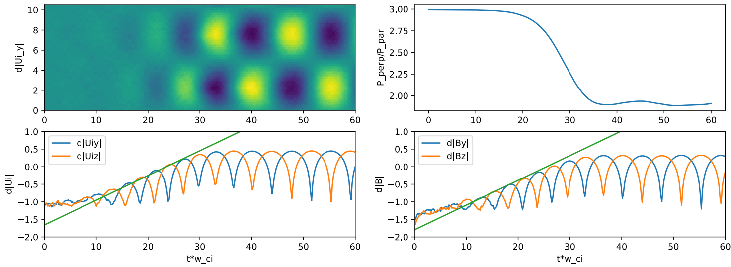
PCAI results:
- Transverse velocity and magnetic field components grow from noise (left-hand Alfvén waves).
- Agree with linear theory for these parameters (\(\gamma/\Omega_{ci} =0.162\)).
- Pressure anisotropy decreases via wave-particle interaction until saturation.
When we add a 20% density fraction of a minor species of alpha particles (\(\text{He}^{2+}\)), the growth rate is found to be smaller. \[ Z_\alpha = 2, M_\alpha = 4, \frac{T_{\alpha\parallel}}{T_{p\parallel}} = 2, \frac{T_{\alpha\perp}}{T_{\alpha\parallel}} = \frac{T_{p\perp}}{T_{p\parallel}} = 3, \frac{N_\alpha}{N_p} = 0.2, Z_\alpha N_\alpha + Z_p N_p = 1 \]
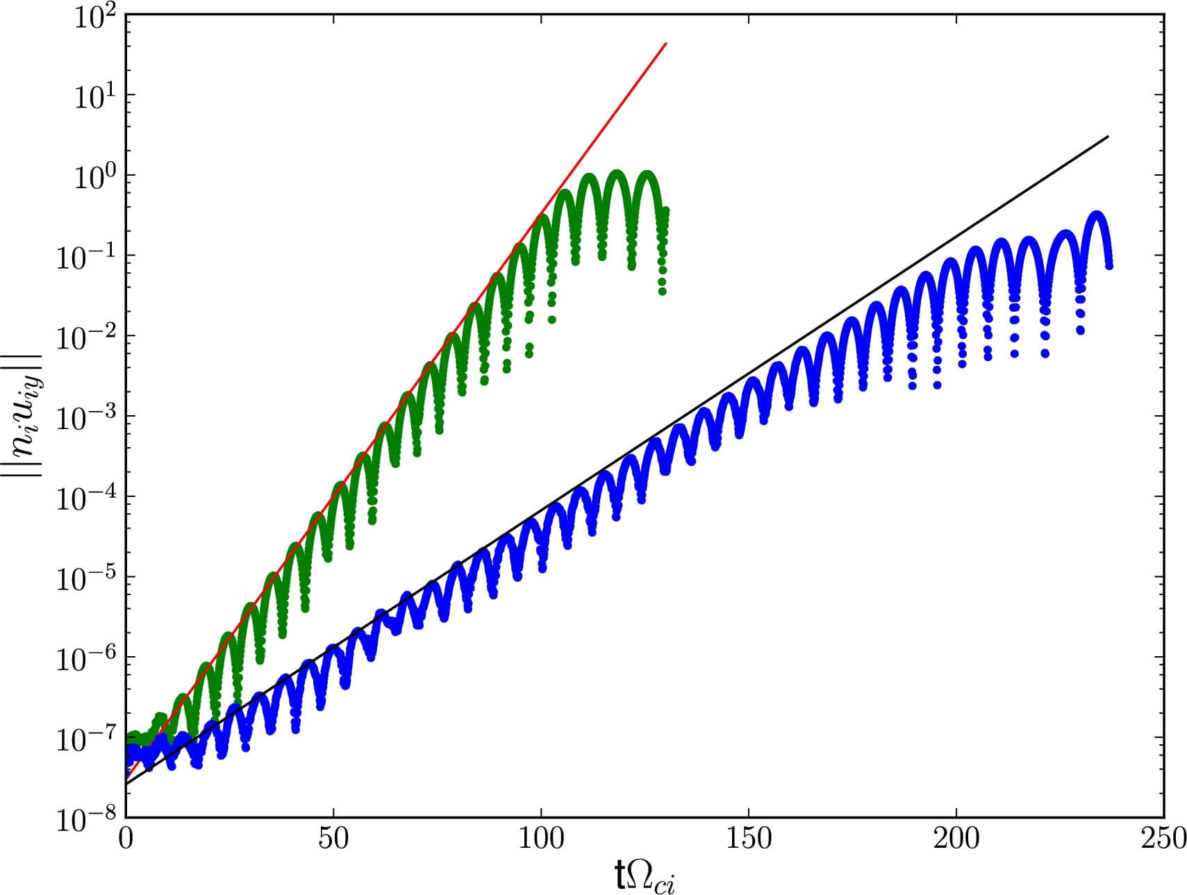
The growth rates across a range of \(\beta\) and anisotropy can be computed and compared with a linear dispersion solver, e.g. HYDROS.
30.8.2 Landau Damped Ion Acoustic Wave
The fundamental electrostatic mode in the hybrid-PIC model is the ion acoustic wave. This is also driven by pressure perturbations. In fluid models (e.g. Hall MHD), this wave is undamped. However, in the hybrid-PIC, Landau resonance damps the wave and locally flattens ion VDF, which is analogous to electron Landau damping of Langmuir oscillations.
The dispersion relation is \[ \frac{dZ(\zeta)}{\mathrm{d}\zeta} = 2\frac{T_i}{T_e},\quad \zeta\equiv \frac{\omega-i\gamma}{kv_{\text{th},i}} \]

The nominal simulation parameters are: \[ T_i = 1/3,\, \gamma=5/3,\, c_s = \sqrt{\gamma T_e/m_i} = 1,\, k_x = \pi/8,\, \delta n = 2\times 10^{-2} \]
Results for nominal parameters
- Damping rate: \(\gamma = -0.0932\).
- Initial perturbation damps to noise floor. Noise can be reduced by:
- Use more particles/cell (noise \(\sim 1/\sqrt(N_p)\)).
- Binomial smoothing/higher order shape functions.
- Using low-discrepancy quasi-Random numbers to seed particles (noise \(\sim 1/N_p\)).
- Most efficient: Delta-F (See Section 29.5).
30.8.3 Magnetic Reconnection Island Coalescence
Magnetic islands are 2D versions of flux-ropes. Here we set a self-driven reconnection problem of coupling of ideal island motion to micro-scale reconnection physics. Ion kinetic effects are crucial in reconnection studies.
Unstable Fadeev island equilibrium: the magnetic field \(\mathbf{B}\) is given by \(\nabla\times\mathbf{A}\), where in this setup we only need \[ A_y = -\lambda B_0 \ln[\text{cosh}(z/\lambda) + \epsilon\cos(z/\lambda)] \] and the density is given by \[ n = n_0(1-\epsilon^2)/[\text{cosh}(z/\lambda) + \epsilon\cos(z/\lambda)]^2 + n_b \]
The pressure balance gives \[ \beta = \frac{2\mu_0 n_0 k_B (T_{i0}+ T_{e0})}{B_0^2} = 1 \]
The nominal simulation parameters are: \[ \lambda = 5d_i,\, \epsilon = 0.4,\, n_b = 0.2n_0,\, T_i/T_e = 1,\, \eta = 10^{-3},\, \eta_H = 5\times10^{-3},\, \gamma = 1 \] and for the numerical parameters, we have a 2D space with \(256\times128\) cells, 50 particles/cell, \(\Delta t\Omega_{ci} = 0.005\).

30.8.4 Collisionless Shock
This is a 2D magnetospheric shock problem, with a \(M_A = 11.4\) shock injected from the right (open) boundary and a reflecting left boundary to drive the collisionless shock.