23 Ionosphere
Ionosphere is like a transition region from neutral gas to plasma. Therefore, collisions as well as kinetic effects gradually become important as we go down from space. Section 9.8 presents some basic physics related to the collisional effect in the ionosphere. This chapter presents the maths for understanding the electromagnetic processes in the ionosphere.
23.1 Derivation of Ionospheric Electrodynamics
To derive the conventional equations of ionospheric electrodynamics from first-principle plasma physics, we start with the exact time-dependent multi-fluid equations for each species and systematically apply the appropriate quasi-steady-state approximations (Song et al. 2001; Vasyliūnas 2012).
23.1.1 The Fundamental Plasma and Maxwell’s Equations
The exact description of the electromagnetic field and the plasma is governed by Maxwell’s equations and the velocity-moment equations derived from the kinetic equations for each species \(\alpha\) (electrons \(e\), ions \(i\), and neutrals \(n\)).
Maxwell’s Equations: - Faraday’s Law: \[\frac{\partial \mathbf{B}}{\partial t} = -c\nabla \times \mathbf{E}\] - Ampère’s Law (with displacement current): \[\frac{\partial \mathbf{E}}{\partial t} = -4\pi \mathbf{J} + c\nabla \times \mathbf{B}\]
Plasma Evolution Equations: The species-specific momentum conservation equation for species \(\alpha\) is: \[ m_\alpha n_\alpha \frac{\partial \mathbf{v}_\alpha}{\partial t} + \nabla\cdot\pmb{\kappa}_\alpha - m_\alpha n_\alpha \mathbf{g} = n_\alpha q_\alpha\left( \mathbf{E} + \frac{1}{c}\mathbf{v}_\alpha \times \mathbf{B} \right) + \mathbf{R}_\alpha \tag{23.1}\] where \(n_\alpha\) is the number density, \(m_\alpha\) is the mass, \(\mathbf{v}_\alpha\) is the velocity, \(q_\alpha\) is the charge (\(q_i = e, q_e = -e\)), \(\pmb{\kappa}_\alpha\) is the kinetic pressure tensor, \(\mathbf{g}\) is gravity, and \(\mathbf{R}_\alpha\) represents the collisional momentum transfer.
23.1.2 Multi-Fluid Definitions and Evolution Equations
Assuming quasi-neutrality (\(n_e \approx n_i = n\)), we define the single-fluid plasma variables: - Plasma mass density: \(\rho = n m_i + n m_e \approx n m_i\) - Plasma bulk velocity: \(\mathbf{V} \approx \mathbf{v}_i + \frac{m_e}{m_i} \mathbf{v}_e\) - Current density: \(\mathbf{J} = ne(\mathbf{v}_i - \mathbf{v}_e)\)
Plasma Bulk Flow Equation: Summing the momentum equations for ions and electrons yields the evolution equation for the plasma bulk flow. The electromagnetic forces resolve to the Lorentz force, and the sum of the collision terms \(\mathbf{R}_i + \mathbf{R}_e\) represents the total drag against the neutral background: \[ \frac{\partial}{\partial t}\left( \rho\mathbf{V} \right) + \nabla\cdot\pmb{\kappa} - \rho\mathbf{g} = \frac{1}{c}\mathbf{J}\times\mathbf{B} - n m_i \nu_{in}\left( \mathbf{V} - \mathbf{V}_n \right) \tag{23.2}\] where \(\nu_{in}\) is the ion-neutral collision frequency and \(\mathbf{V}_n\) is the neutral wind velocity.
Generalized Ohm’s Law (Current Density Evolution): Subtracting the electron momentum equation from the ion momentum equation (weighted by charge-to-mass ratios) yields the evolution of the current density. Under the assumption \(m_e \ll m_i\), the electron dynamics dominate1, leading to: \[ \frac{\partial \mathbf{J}}{\partial t} = \frac{ne^2}{m_e}\left( \mathbf{E} + \frac{1}{c}\mathbf{V}\times\mathbf{B} - \frac{\mathbf{J}\times\mathbf{B}}{nec} \right) + \left( \frac{\delta \mathbf{J}}{\delta t} \right)_\mathrm{coll} \tag{23.3}\] In the ionospheric regime, the collision term simplifies to: \[ \left( \frac{\delta \mathbf{J}}{\delta t} \right)_\mathrm{coll} \simeq -\nu_e \mathbf{J} \] where \(\nu_e = \nu_{ei} + \nu_{en}\) is the total electron collision frequency.
23.1.3 Quasi-Steady-State Approximations
To transition to the conventional steady-state formulations, we apply two main approximations under specific physical conditions:
Neglecting High-Frequency Oscillations: For phenomena with spatial scales much larger than the electron inertial length \(\lambda_e\) and timescales much longer than the inverse plasma frequency \(\omega_p^{-1}\), we can neglect the temporal derivatives of the current density and electric field: \[\frac{\partial \mathbf{J}}{\partial t} \approx 0, \quad \frac{\partial \mathbf{E}}{\partial t} \approx 0\]
Neglecting Inertia and Other Forcings: Assuming slow plasma acceleration and neglecting pressure gradients and gravity relative to electromagnetic and collisional forces, the bulk flow equation (Equation 23.2) reduces to a strict stress balance: \[0 \simeq \frac{1}{c}\mathbf{J}\times\mathbf{B} - n m_i \nu_{in}\left( \mathbf{V} - \mathbf{V}_n \right) \tag{23.4}\] Simultaneously, the generalized Ohm’s law (Equation 23.3) simplifies to: \[0 \simeq \mathbf{E} + \frac{1}{c}\mathbf{V}\times\mathbf{B} - \frac{\mathbf{J}\times\mathbf{B}}{nec} - \frac{m_e\nu_e}{ne^2}\mathbf{J} \tag{23.5}\]
Alternatively, the stress-balance in the perpendicular direction can be expressed in terms of the drift velocities: \[0 = c\frac{\mathbf{E}}{B} + \mathbf{V} \times \hat{\mathbf{b}} - \frac{\nu_{in}}{\Omega_i}(\mathbf{V} - \mathbf{V}_n) \tag{23.6}\] where \(\hat{\mathbf{b}} = \mathbf{B}/B\) is the unit vector along the magnetic field and \(\Omega_i = eB/(m_i c)\) is the ion gyrofrequency. This describes the \(\mathbf{E} \times \mathbf{B}\) drift modified by collisional drag with neutrals.
23.1.4 Deriving the Ionospheric Ohm’s Laws
To establish the relationship between current and the electric field, we express the equations in the frame of the neutral wind. First, we solve the stress balance equation (Equation 23.4) for the relative velocity: \[ \mathbf{V} - \mathbf{V}_n = \frac{1}{cn m_i \nu_{in}}\mathbf{J}\times\mathbf{B} \] Substituting \(\mathbf{V} = \mathbf{V}_n + \frac{1}{cn m_i \nu_{in}}\mathbf{J}\times\mathbf{B}\) into the reduced Ohm’s law (Equation 23.5) yields: \[ 0 = \left(\mathbf{E} + \frac{1}{c}\mathbf{V}_n \times \mathbf{B}\right) + \frac{(\mathbf{J}\times\mathbf{B})\times\mathbf{B}}{c^2 n m_i \nu_{in}} - \frac{\mathbf{J}\times\mathbf{B}}{nec} - \frac{m_e\nu_e}{ne^2}\mathbf{J} \] Defining the electric field in the frame of the neutral atmosphere as \(\mathbf{E}^\prime \equiv \mathbf{E} + \frac{1}{c}\mathbf{V}_n\times\mathbf{B}\), and using the vector identity \((\mathbf{J}\times\mathbf{B})\times\mathbf{B} = -\mathbf{J}_\perp B^2\), we decompose the equation into components parallel and perpendicular to the magnetic field.
Parallel Component: \[0 = \mathbf{E}_\parallel^\prime - \frac{m_e\nu_e}{ne^2}\mathbf{J}_\parallel \implies \mathbf{J}_\parallel = \sigma_\parallel \mathbf{E}_\parallel^\prime\] where the parallel conductivity is \(\sigma_\parallel = \frac{ne^2}{m_e\nu_e}\).
Perpendicular Component: Defining the effective Pedersen and Hall resistivities: \[\rho_P = \frac{B^2}{c^2 n m_i \nu_{in}} + \frac{m_e \nu_e}{ne^2}, \quad \rho_H = \frac{B}{nec}\] The perpendicular component of the equation becomes: \[\mathbf{E}_\perp^\prime = \rho_P \mathbf{J}_\perp + \rho_H \left( \mathbf{J}_\perp \times \hat{\mathbf{b}} \right)\] Inverting this system of equations yields the conventional ionospheric Ohm’s law: \[\mathbf{J}_\perp = \sigma_P \mathbf{E}_\perp^\prime + \sigma_H\left( \hat{\mathbf{b}} \times \mathbf{E}_\perp^\prime \right) \tag{23.7}\] where the Pedersen and Hall conductivities are: \[\sigma_P = \frac{\rho_P}{\rho_P^2 + \rho_H^2}, \quad \sigma_H = \frac{\rho_H}{\rho_P^2 + \rho_H^2}\]
(Note: If we instead chose to eliminate the neutral velocity \(\mathbf{V}_n\) from the coupled electron and ion force balance equations, we would obtain the three-fluid Ohm’s law in the plasma frame, describing the current relative to the plasma bulk flow \(\mathbf{V}\). However, expressing the current in the neutral wind frame is conventional for modeling the ionosphere.)
23.1.5 Deriving the Electric Potential and Current Continuity
To solve for the spatial distribution of the electric field, we apply two final steady-state approximations to Maxwell’s equations:
Potential Electric Field: Neglecting wave propagation effects (meaning magnetic variations are slow relative to Alfvén times), Faraday’s law simplifies to \(\nabla \times \mathbf{E} \approx 0\), which allows us to express the electric field as the gradient of a scalar potential: \[\mathbf{E} = -\nabla \Phi\]
Current Continuity: Dropping the displacement current from Ampère’s law (\(c\nabla \times \mathbf{B} = 4\pi \mathbf{J}\)) implies that the current density is solenoidal: \[\nabla \cdot \mathbf{J} = 0\]
Substituting the potential representation and the conventional Ohm’s law (\(\mathbf{J} = \pmb{\sigma} \cdot \mathbf{E}'\)) into the current continuity equation yields: \[ \nabla \cdot \left[ \pmb{\sigma} \cdot \left( -\nabla\Phi + \frac{1}{c}\mathbf{V}_n \times \mathbf{B} \right) \right] = 0 \] which gives the final 3D elliptic equation for the electric potential: \[ \nabla \cdot (\pmb{\sigma} \cdot \nabla \Phi) = \frac{1}{c} \nabla \cdot \left[ \pmb{\sigma} \cdot \left(\mathbf{V}_n \times \mathbf{B}\right) \right] \tag{23.8}\] Here, the conductivity tensor \(\pmb{\sigma}\) in the coordinate system aligned with \(\mathbf{B}\) is: \[ \pmb{\sigma} = \begin{pmatrix} \sigma_P & -\sigma_H & 0 \\ \sigma_H & \sigma_P & 0 \\ 0 & 0 & \sigma_\parallel \end{pmatrix} \]
Integrating this 3D relation along the magnetic field line over the height of the conducting layer yields the 2D height-integrated potential equation used as a boundary condition in magnetosphere-ionosphere coupling models.
23.1.6 When These Fails
The conventional equations of ionospheric electrodynamics fail to capture the underlying physics when they are used to describe dynamic developments, temporal sequences, and causal relationships (Vasyliūnas 2012). Because these equations are derived by neglecting local dynamical terms—such as time derivatives, plasma acceleration, and pressure gradients—they are only rigorously valid for describing quasi-steady-state equilibrium conditions that involve slow variations.
Specifically, the traditional equations break down or fail to accurately reflect physical reality in the following scenarios:
- Determining Cause and Effect in Plasma Flow: The conventional equations act merely as relations between quantities at a given time and cannot specify how a system evolves. Traditional verbal descriptions often incorrectly interpret the equations to mean that an imposed electric field causes plasma bulk flow via \(E \times B\) drift. However, solving the complete initial-value equations reveals the opposite is true: plasma flows produce electric fields, but electric fields do not produce flows.
- Fast Time Scales and Small Spatial Scales: To simplify calculations, the conventional equations drop time derivatives, including the displacement-current term in Maxwell’s equations. Consequently, they fail for high-frequency phenomena (approaching the plasma frequency) and on small spatial scales (shorter than the electron inertial length, which is roughly tens of meters). On these short time scales, dynamic processes like charge separation and accumulation become significant and cannot be ignored.
- Wave Propagation and Field Line Readjustments: The traditional equations assume the electric field has a negligible curl and can be treated as a scalar potential. This assumption fails to capture the physics when the time scale of magnetic variations is not significantly longer than the spatial scale divided by the Alfvén speed. Furthermore, the conventional assumption that magnetic field lines are near-equipotential is often mischaracterized as a spontaneous “mapping” of electric fields; in reality, differences in flow and electric fields are communicated dynamically via MHD (Alfvén) waves propagating back and forth along the field lines.
- The Neutral-Wind Dynamo: Conventional models frequently assume that neutral winds generate permanent electric currents directly because collisions affect ions differently than electrons. The complete physical equations reveal that this direct process only creates a brief, transient current that quickly dies away. In reality, the traditional equations obscure the fact that a permanent dynamo current only arises from spatial gradients in the plasma flow that deform the magnetic field, with the current ultimately arising to match the curl of this deformed field.
- Momentum and Mechanical Stress: Because the conventional approach drops acceleration terms, it reduces ionospheric electrodynamics to a problem of electrostatic or magnetostatic balance. It fails to capture the fundamental mechanism that bulk plasma flow carries linear momentum, which must be physically added to the plasma by mechanical stresses or the Lorentz force of an external current, rather than simply manifesting out of an electric field.
23.2 Current Systems
Electric fields associated with the viscous interaction and reconnection-driven plasma flow are transmitted along field lines to the ionosphere where they drive currents through the ionosphere. The high latitude FAC are known as region-1 currents, while the lower latitude currents are called region-2 currents. The ionospheric current connecting these two FAC systems flows parallel to the projected electric field and is called the Pedersen current. Since the Pedersen current flows through a resistive ionosphere in the direction of the electric field it causes Ohmic heating \(\mathbf{j}\cdot\mathbf{E}>0\). The two shells of FAC form a solenoid so that the magnetic perturbations they create are confined to the region between them and cannot be detected on the ground. Because of the interaction of the motion of ionized gases with the neutral atmosphere, the ions and electrons undergo different drift motion. Ions, due to higher collision rates with the neutral atmosphere, have a component of motion perpendicular to the \(\mathbf{E}\times\mathbf{B}\) drift direction, while the electrons generally follow \(\mathbf{E}\times\mathbf{B}\). The non-dissipative (\(\mathbf{j}\cdot\mathbf{E}=0\)) Hall current flows at right angles to both the electric and magnetic fields. The magnetic effects of the Hall current driven by the region-1 and 2 currents can be observed on the ground and are known as the DP-2 current system.2
In the context of ionospheric energy dissipation, the different current systems can be classified into two types based on how energy is processed.
- If the ionospheric motion and dissipation is coupled directly to the solar wind, the system is said to be “directly-driven”. The directly-driven process manifests itself as the DP-2 (two cell pattern) ionospheric current system.
- If magnetic energy is first stored in the tail lobes and then released some time later, driving additional convection and field-aligned and ionospheric currents, it is called “unloading”, and is associated with the DP-1 (substorm current wedge) current system.
Both processes cause precipitation of charged particles that also deposit energy in the atmosphere.
The characteristic feature of the driven DP-2 current system is the existence of the eastward and westward electrojets flowing toward midnight along the auroral oval. Rough measures of the strength of these currents are the auroral upper (AU) and auroral lower (AL) indices. These are respectively the largest positive northward magnetic perturbation (H) measured on the ground under the eastward electrojet by any magnetic observatory in the afternoon to dusk sector, and the largest negative southward perturbation measured in the late evening to morning sector. Both AU and AL begin to grow in intensity soon after the IMF turns southward and dayside reconnection begins. The characteristic feature of the unloading DP-1 current system is the sudden development of an additional westward current that flows across the bright region of the expanding auroral bulge. This is the ionospheric segment of the substorm current wedge. The onset of this current is recorded in the AL index as a sudden decrease, corresponding to an increase in intensity of the westward current.
23.3 M-I Coupling
Ionospheric properties, principally conductivity, provide boundary conditions for magnetospheric convection, and the ionosphere is often treated as a passive part of the system. Especially during substorms, however, the boundary conditions change in a time-dependent and spatially localized fashion, allowing ionospheric feedback that can alter the magnetospheric dynamics. The coupling from the ionospheric perspective differs primarily in that the ionospheric conductance is anisotropic due to the influence of the neutral atmosphere, involving Hall as well as Pedersen conductivity. These conductivities are altered both by the connecting currents and the precipitating electrons associated with upward field-aligned currents, which increase Pedersen conductivity and field line tying. An important role is also played by field-aligned electric fields, set up locally, primarily in upward field-aligned current regions, which are the cause of auroral intensifications and, specifically auroral arcs.
For magnetosphere simulations, the simplest inner boundary is treated as a conducting sphere (\(\mathbf{B}_\text{normal}=0\), \(\mathbf{E}=\mathbf{v}=0\)). However, this is often not realistic enough to reveal the nature. In magnetosphere simulations, the location of tail main reconnection site will be closer to the Earth by simply applying a conducting boundary. The next level extension is to employ a magnetospheric-ionospheric electrostatic coupling model. This means that we seek nonzero \(\mathbf{E}\) and \(\mathbf{v}\) at the inner boundary. The inner boundary, where the MHD quantities are connected to the ionosphere, is taken to be a shell of radius \(r_\text{in}\) (e.g. \(r_\text{in}\sim 3\,\text{R}_\text{E}\)). The ionosphere locates at \(r_\text{ion}\sim 1000\,\text{km}\sim 0.15\,\text{R}_\text{E}\). Ideally \(r_\text{in}\) shall be as close to \(r_\text{ion}\) as possible, but typically it is restricted by computational limitations, such as extraneously high Alfvén speeds and very large \(\mathbf{B}\) field gradients closer to the Earth. Inside this shell we do not solve the governing equations (MHD/PIC/Vlasov), but assume a static dipole field. The important physical processes within the shell are the flow of field-aligned currents (FACs) and the closure of these currents in the ionosphere. At each time step,
- The magnetospheric FACs are mapped along the field lines from the inner boundary to the ionosphere assuming \(j_\parallel/B=\text{const.}\), which are the input to the ionospheric potential equation (Raeder et al. 1995) \[ \nabla\cdot(\pmb{\Sigma}\cdot\nabla\Phi) = -j_\parallel\sin I \tag{23.9}\] where \(\pmb{\Sigma}\) is the conductance tensor, \(\Phi\) is the electric potential, \(j_\parallel\) is the mapped FAC density with the downward considered positive and corrected for flux tube convergence, and \(I\) is the inclination of the dipole field at the ionosphere, \(\sin I=\cos(\frac{\pi}{2}-I)=\hat{b}\cdot\hat{r}\). The derivation from the charge conservation can be found in Section 9.8.7. There is another form derived by [Wolf 1983]: \[ \nabla_\perp\cdot \begin{pmatrix} \Sigma_P/\cos^2\delta & -\Sigma_H/\cos\delta \\ \Sigma_H/\cos\delta & \Sigma_P \end{pmatrix} \cdot\nabla_\perp\Phi = j_\parallel\cos\delta \tag{23.10}\] where \(\delta\) is the magnetic field dip angle (the angle between the magnetic field vector and the vertical radial direction): \[ \cos\delta = -2\frac{\cos\theta}{\sqrt{1+3\cos^2\theta}} \] for the northern hemisphere, where \(\theta\) is the polar angle (magnetic colatitude).
The relation between the two forms Equation 23.9 and Equation 23.10 lies in their coordinate representation of the height-integrated current conservation. In Equation 23.9, \(I\) is the magnetic inclination (the angle the magnetic field makes with the horizontal). In Equation 23.10, \(\delta\) is the dip angle measured from the vertical (radial direction). Since they are complementary, \(\cos\delta = \sin I\). Thus, the right-hand sides of the two equations are equivalent (subject to the convention for the direction of \(j_\parallel\)). The left-hand side of Equation 23.9 is written in coordinate-free tensor form, where the conductance tensor \(\pmb{\Sigma}\) maps the horizontal electric field to the horizontal current. In the spherical coordinate basis \((\hat{\pmb{\theta}}, \hat{\pmb{\phi}})\) (where \(\hat{\pmb{\theta}}\) points southwards and \(\hat{\pmb{\phi}}\) points eastwards), the tilted magnetic field yields the horizontal conductance matrix shown in Equation 23.10: \[ \pmb{\Sigma}_h = \begin{pmatrix} \Sigma_P/\cos^2\delta & -\Sigma_H/\cos\delta \\ \Sigma_H/\cos\delta & \Sigma_P \end{pmatrix} \] (Note: The top-right term \(-\sigma_H\cos\delta\) in the original formulation has been corrected to \(-\Sigma_H/\cos\delta\) to maintain proper scaling for the horizontal Hall current and represent height-integrated conductances consistently). Thus, the two equations are completely equivalent representations of the same 2D current conservation equation.
- Equation 23.9 is solved on the surface of a sphere \(r=r_\text{ion}\). Commonly there are two types of boundary conditions: (1) \(\Phi=0\) at the equator (Raeder et al. 1995), or (2) constant potential at or near the low‐latitude boundary (e.g. LFM, BATSRUS). From here, one can either choose a static analytic model of Hall and Pederson conductance that accounts for multiple physics, or simply adopt a uniform Pederson conductance, or the height-integrated conductivity, \(\Sigma_p = 5\,\text{Siemens}\), while the Hall conductance \(\Sigma_H\) is assumed to be zero. The latter one is simplified to solve \[ \nabla^2\Phi = -j_\parallel\sin I/\Sigma_p \]
A more realistic conductance requires considering EUV and diffuse auroral contributions (???) as well. The solar EUV contribution to \(\pmb{\Sigma}\) is considered constant in time, but naturally it varies with the solar zenith angle. For example, the empirical formulas by [Moen and Brekke 1993] can be used. The solar EUV radiation is approximated by the 10.7 cm radio flux (commonly known as F10.7), a widely used proxy solar UV activity, whose standard values is taken to be \(100\times 10^{-22}\,\text{W}/\text{m}^2\).
The total conductance can be then expressed as \[ \Sigma_{P,H} = \sqrt{(\Sigma_{P,H}^{e-})^2 + (\Sigma_{P,H}^{\text{UV}})^2} \]
This is because \(\sigma_{P,H}\propto n_e\), which in a stationary state is proportional to the square root of the production rate, and it is the production rates that can be summed linearly. (???)
Does this look well? Not yet. We know that while the high‐latitude ionospheric convection is driven by the solar wind and magnetosphere interaction, at lower latitudes atmospheric neutral winds start to dominate. The next level approximation needs to take this into account. Because there is a gap between \(r_\text{ion}\) and \(r_\text{in}\), the ionospheric footprint of their grid has a low‐latitude boundary somewhere in the midlatitudes, e.g., 45° when \(r_\text{in}\sim 2\,\text{R}_\text{E}\) (Figure 23.1). Global magnetospheric models, unless they are fully coupled to models of the inner magnetosphere and the ionosphere, lack details of the ionospheric convection at latitudes equatorward of their low‐latitude ionospheric boundary. To some extent, such details can be translated to the global model via the low‐latitude boundary condition used to solve Equation 23.10. The easy way is to set the ionospheric potential to zero everywhere on the boundary. This corresponds to no flow across the boundary in the ionosphere or the inner boundary of the magnetosphere simulation in the equatorial plane. The choice of this boundary condition is usually justified by the argument that it helps to shield the inner magnetosphere from the cross‐tail electric field.
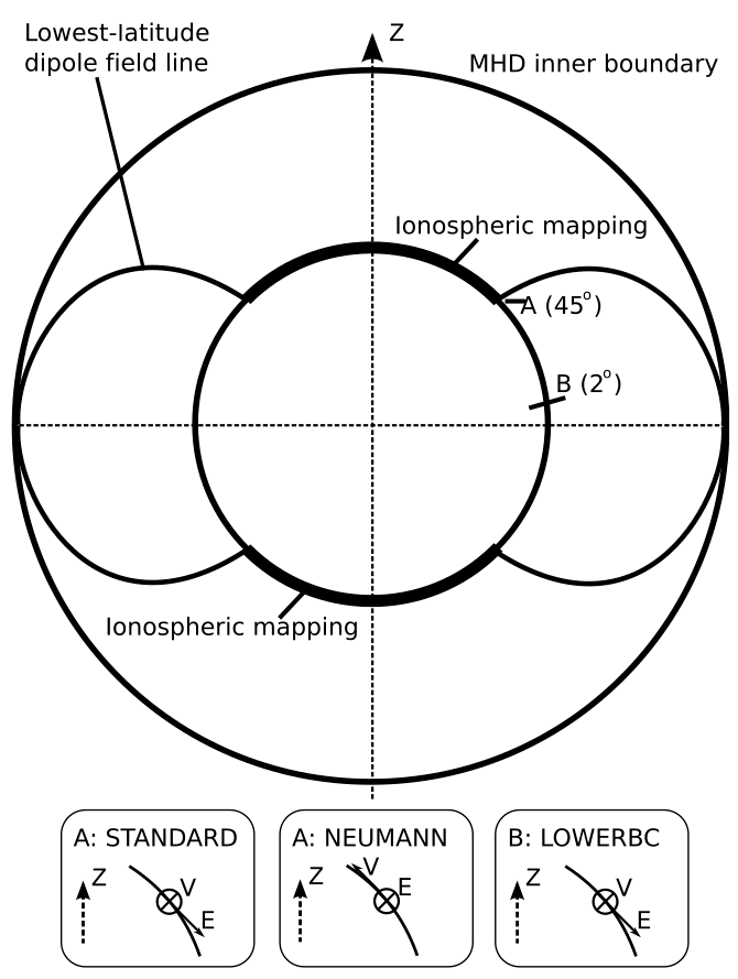
(Merkin and Lyon 2010) tested three different boundary conditions for the potential equation:
- STANDARD: Dirichlet, the potential at the low‐latitude boundary is set to zero.
- NEUMANN: the electric field component normal to the low‐latitude boundary was set to zero. This condition requires all ionospheric plasma to move normal to the boundary.
- LOWERBC: Dirichlet, but the location of the low‐latitude boundary was moved to 2° above the equator, thus allowing the plasma to move across the magnetosphere inner boundary. (???) Equation 23.11 is singular at \(\theta=\pi/2\), which is why the calculation has to stop just short of the equator. (???)
Sparse linear algebra, GMRES together with an imcomplete LU preconditioner (default for many modern solvers) are usually applied to solve the potential equation. This is generally an easy equation to solve mathematically.
Once the potential equation is solved the ionospheric potential is mapped back to the \(r_\text{in}\) shell and used as a boundary condition for the magnetospheric flow by taking \(\mathbf{v}=(-\nabla\Phi)\times\mathbf{B}/B^2\).
23.3.1 Caveats
- The mapping assumes conservation, which is not perfect. In practice \(r_\text{in}\sim 4\,\text{R}_\text{E}\) is a minimum requirement for reasonable FACs.
- Most numerical codes couples a Cartesian grid to a spherical ionosphere grid, while some couples a spherical grid to a spherical grid. For magnetosphere simulations we need a relatively simple but super fast electric potential solver, therefore structured mesh is often adopted. If a spherical grid is used, care must be taken near the pole since it is a singular from the grid but not physics. Equation 23.10 under spherical coordinates is written as
\[ \begin{aligned} \frac{1}{\sin\theta}&\frac{\partial}{\partial\theta}\Big[ \sin\theta\frac{\Sigma_P}{\cos^2\delta}\frac{\partial\Phi}{\partial\theta} - \frac{\Sigma_H}{\cos\delta}\frac{\partial\Phi}{\partial\phi} \Big] \\ + &\frac{\partial}{\partial\phi}\Big[ \frac{\Sigma_P}{\sin^2\theta}\frac{\partial\Phi}{\partial\phi}+\frac{\Sigma_H}{\sin\theta\cos\delta}\frac{\partial\Phi}{\partial\theta} \Big] = j_\parallel R^2\cos\delta \end{aligned} \tag{23.11}\]
Be careful about distinguishing \(E_\parallel\) and \(j_\parallel\). \(E_\parallel = 0\) from advection and Hall terms, but \(j_\parallel=\nabla\times\mathbf{B}\cdot\hat{b}/\mu_0\) can be nonzero at the MHD inner boundary.
How important it is to use a more realistic conductance model? (Merkin and Lyon 2010) shows that different BCs may give > 10% CPCP values, but I have no clue about the effect of a more complicated conductance.
23.4 Ionosphere Modeling
- What equation set is the model solving? How is the model solving them? What is being neglected?
- What species are included? How is the chemistry solved?
- Parameterizations in things such as heating, cooling, viscosity, conduction, chemistry, diffusion, collision, absorption, ionization cross sections, reaction rates…
- How are upper and lower boundaries treated? How is the pole or the open/closed field-line boundary treated?
- How are electrodynamics considered? How is the aurora specified? How is the magnetospheric electric field imposed? Is ion precipitation considered?
For an ionosphere, a magnetic field-aligned grid is often used. This is complicated by the non-orthogonal nature of the magnetic field coordinate system. Assumptions are made.
How to solve each direction (coupled or independently)? For the ionosphere, along the field-line is treated differently than across the field-lines.
As the equations of motion are solved for, the source terms must be added. How to treat these with respect to solving in the different directions?
Build a simple 1D ionosphere model is easy (CAN I MAKE ONE MYSELF?).
Steady-state - assume \(\partial \mathbf{X}/\partial t = 0\). Strangly, this is applied in situations in which the value can change on a time scale much faster than the time-step. For example, the ion velocity is often assumed to be steady-state. Ion chemistry is sometimes assumed to be steady-state.
23.4.1 Chemistry
\[ \frac{\partial N}{\partial t} = S - L \] where \(N\) is the number density of the species, \(S\) represents the sources and \(L\) represents the losses. Losses can almost always be expressed as: \[ L = RMN \] where \(R\) is the reaction rate, \(M\) is the density of the species it is reacting with.
For a steady-state, \[ \begin{aligned} S - L &= 0 \\ N &= \frac{S}{RM} \end{aligned} \]
This is quite stable, but can be very wrong in regions of slowly changing ion densities, such as in the F-region. This is perfect for the E-region, though. It is quite easy to implement in a simple environment, but can be much more complicated as non-linear terms are include (recombination, in which \(M\) can depend on \(N\)).
An explicit time step chemistry is trivial to implement in almost all situations, but it is also the least stable, since the loss terms can become larger than the source terms and the density can quickly be driven to negative values. Subcycling can help with this, but not always.
An implicit time step chemistry is relatively stable and easier to implement than steady-state. For example in GITM, there is a blend between sub-cycling and a simplified implicit scheme that switches depending on the size of the loss term compared to the density.
Now we need to also look at the source terms. The ionization rates can be obtained from \(Q_\text{EUV}\) and substituting \(\sigma_s^i \lambda\) instead of \(\sigma_s^a\lambda\) (not in \(\tau\)). [Schunk and Nagy] Chapter 8 list a bunch of chemical equations.
After that, we write down all the sources and losses, decide a time-stepping scheme, and run the model. However, if we don’t have any ion advection, the F-region will just build and build!
23.4.2 Ion Advection
In the simplest form, we assume an advection speed and let the densities advect upward and downward.
23.5 Ionosphere Waveguide
The ionosphere waveguide refers to the phenomenon in which certain radio waves can propagate in the space between the ground and the boundary of the ionosphere. Because the ionosphere contains charged particles, it can behave as a conductor. The planet operates as a ground plane, and the resulting cavity behaves as a large waveguide. This is closely related to the concept of skin depth in EM and the cutoff in wave propagation.
At Earth, extremely low frequency (ELF) (< 3 kHz) and very low frequency (VLF) (3–30 kHz) signals can propagate efficiently in this waveguide. For instance, lightning strikes launch a signal called radio atmospherics, which can travel many thousands of kilometers, because they are confined between the Earth and the ionosphere. The round-the-world nature of the waveguide produces resonances, like a cavity, which are at \(\sim 7\) Hz.
A brief introduction can be found on wiki.
23.6 Incoherent Scatter Radar
Longitudinal modes:
- Langmuir wave
- Ion acoustic wave
Cascading Langmuir turbulence
dispersive, kinetic Alfven waves –> optical manifestation of dispersive bursts