14 Kinetic MHD
This is taken from the hand-written lecture notes from Prof. Alexander Schekochihin. Theoretical physicists love CGS units, but I tend to use SI units here. In later part of the note, there may be mixed units, so be careful.
We start by showing how for magnetized, weakly collisional plasmas (\(\nu_\text{colli} \ll \Omega_s\), \(r_L\ll \lambda_\text{mfp}\), where \(\lambda_\text{mfp}\) is the mean free path), low-frequency (\(\omega \ll \Omega_s\)), long-wavelength (\(kr_L\ll 1\)) dynamics can be decided by a set of equations that look almost like the familiar MHD. We will see later on that the ways in which they are not MHD will profoundly affact the dynamics — indeed we do not fully understand the full implication of this in high-\(\beta\) plasmas. This is consequently one of the frontier topics in theoretical plasma astrophysics.
Let us start from first principles. Any plasma that is going to be of interest to us is described by the Vlasov-Maxwell-Landau system of equations: \[ \frac{\partial f_s}{\partial t} + \mathbf{v}\cdot\nabla f_s + \frac{q_s}{m_s}\Big[\mathbf{E} + \mathbf{v}\times\mathbf{B} \Big]\frac{\partial f_s}{\partial\mathbf{v}} = C(f_s) \tag{14.1}\]
The Maxwell’s equation can be simplified based on our assumptions. \[ \nabla\cdot\mathbf{E} = \epsilon_0 \sum_s q_s n_s,\, n_s=\int \mathrm{d}\mathbf{v}f_s \]
\(\nabla\cdot\mathbf{E}\) is small when \(k^2\lambda_{De}\ll 1\), and this simply gives the quasi-neutrality condition.
\[ \nabla\cdot\mathbf{B} = 0 \]
\[ \frac{\partial\mathbf{B}}{\partial t} = -\nabla\times\mathbf{E} \]
\[ \nabla\times\mathbf{B} = \mu_0\mathbf{j} + \cancel{\epsilon_0\mu_0 \frac{\partial\mathbf{E}}{\partial t}},\, \mathbf{j} = \sum_s n_s q_s \mathbf{u}_s, \mathbf{u}_s = \frac{1}{n_s}\int \mathrm{d}\mathbf{v}\mathbf{v} f_s \]
The displacement current can be neglected since \(\omega\ll kc\) for low frequency waves and non-relativistic motions.
Intuitively, we tend to think of the plasma as a fluid (or a multi-fluid of several species) with some density \(n_s\), velocity \(\mathbf{u}_s\) and perhaps pressure, temperature, etc. This is rooted in our experience with collisional gases (\(\nu\gg \omega\)), which are in local Maxwellian equilibrium: \[ f_s = \frac{n_s}{(\pi v_{\text{th},s}^2)^{3/2}}e^{-\frac{(\mathbf{v}-\mathbf{v}_s)^2}{v_{\text{th},s}^2}},\, v_{\text{th},s} = \sqrt{\frac{2k_B T_s}{m_s}} \] where \(n_s, \mathbf{u}_s\) and \(T_s\) are governed by fluid equations.
With this desire to think of plasmas as fluid, let us break the motion of the particles into two parts: \[ \mathbf{v} = \mathbf{u}_s(t,\mathbf{r}) + \mathbf{w} \] where \(\mathbf{u}_s\) represents the mean velocity of species \(s\) (fluid-like description) and \(\mathbf{w}\) represents the “peculiar” velocity or internal motion (kinetic description). This amounts to a transformation of variables \[ (t,\mathbf{r},\mathbf{v}) \rightarrow (t,\mathbf{r},\mathbf{w}),\quad\mathbf{w} = \mathbf{v} - \mathbf{u}_s(t,\mathbf{r}) \] under which the derivatives in the new basis shall be written as \[ \begin{aligned} \frac{\partial}{\partial t}&\rightarrow \frac{\partial}{\partial t} - \frac{\partial\mathbf{u}_s}{\partial t}\cdot\frac{\partial}{\partial\mathbf{w}} \\ \nabla&\rightarrow \nabla-(\nabla\mathbf{u}_s)\cdot\frac{\partial}{\partial\mathbf{w}} \\ \frac{\partial}{\partial\mathbf{v}}&\rightarrow \frac{\partial}{\partial\mathbf{w}} \end{aligned} \tag{14.2}\]
This can be derived from the chain rule with \[ \begin{aligned} t^\prime &= t \\ \mathbf{r}^\prime &= \mathbf{r} \\ \mathbf{w} &= \mathbf{v} - \mathbf{u}_s(t,\mathbf{r}) \end{aligned} \]
Note that the three variables are independent, for any quantity \(f\), we have \[ \begin{aligned} \frac{\partial f}{\partial t} &= \frac{\partial f}{\partial t^\prime}\cdot\frac{\partial t^\prime}{\partial t} + \frac{\partial f}{\partial \mathbf{r}^\prime}\cdot\frac{\partial\mathbf{r}^\prime}{\partial t} + \frac{\partial f}{\partial\mathbf{w}}\cdot\frac{\partial\mathbf{w}}{\partial t} \\ &= \frac{\partial f}{\partial t} - \frac{\partial\mathbf{u}_s}{\partial t}\cdot\frac{\mathbf{\partial f}}{\partial \mathbf{w}} \end{aligned} \]
Similarly we can derive the other two relations in Equation 14.2. Then the Boltzmann equation becomes \[ \Big( \frac{\partial}{\partial t} + \mathbf{u}_s\cdot\nabla\Big)f_s + (\mathbf{w}\cdot\nabla)f_s + \Big(\frac{q_s}{m_s}\mathbf{w}\times\mathbf{B} +\mathbf{a}_s -\mathbf{w}\cdot\nabla\mathbf{u}_s )\cdot\frac{\partial f_s}{\partial\mathbf{w}} = C(f_s) \tag{14.3}\] where \[ \mathbf{a}_s = \frac{q_s}{m_s}\Big(\mathbf{E} + \mathbf{u}_s\times\mathbf{B} \Big) - \frac{\mathrm{d}\mathbf{u}_s}{\mathrm{d}t} \] and now we always have \(\int \mathrm{d}\mathbf{w}\mathbf{w}f_s = 0\) by definition. The strategy now is to take moments of Equation 14.3. The zeroth-order moment (\(\int \mathrm{d}\mathbf{w}\)) gives \[ \begin{aligned} \int \frac{df_s}{\mathrm{d}t} \mathrm{d}\mathbf{w} + \int (\mathbf{w}\cdot\nabla)f_s \mathrm{d}\mathbf{w} + \int \Big[... \Big]\cdot\frac{\partial f_s}{\partial\mathbf{w}} \mathrm{d}\mathbf{w} = 0 \\ \frac{\mathrm{d}}{\mathrm{d}t}\int f_s \mathrm{d}\mathbf{w} + \cancel{\nabla\cdot\int \mathbf{w}f_s \mathrm{d}\mathbf{w}} - \int (\mathbf{w}\cdot\nabla\mathbf{u}_s)\cdot\frac{\partial f_s}{\partial\mathbf{w}} \mathrm{d}\mathbf{w} = 0 \\ \frac{dn_s}{\mathrm{d}t} + \int f_s \frac{\partial}{\partial\mathbf{w}}\big(\mathbf{w}\cdot\nabla\mathbf{u}_s \big)\mathrm{d}\mathbf{w} = 0 \\ \frac{dn_s}{\mathrm{d}t} + \int f_s \frac{\partial}{\partial w_j}\big(w_i \frac{\partial}{\partial x_i}u_{sj} \big)dw_j = 0 \\ \frac{dn_s}{\mathrm{d}t} + \int f_s \delta_{ij}\frac{\partial}{\partial x_i}u_{sj}dw_j + \int f_s w_i \cancel{\frac{\partial^2 u_{sj}}{\partial x_i \partial w_j}}dw_j = 0 \\ \frac{dn_s}{\mathrm{d}t} + \int f_s \frac{\partial}{\partial x_i}u_{si}dw_i = 0 \\ \frac{dn_s}{\mathrm{d}t} + \nabla\cdot\mathbf{u}_s\int f_s \mathrm{d}\mathbf{w} = 0 \\ \frac{dn_s}{\mathrm{d}t} + (\nabla\cdot\mathbf{u}_s)n_s = 0 \end{aligned} \] or \[ \frac{\partial n_s}{\partial t} + \nabla\cdot(n_s\mathbf{u}_s) = 0 \tag{14.4}\]
The first-order moment (\(\int \mathrm{d}\mathbf{w}m_s\mathbf{w}\)) gives \[ \nabla\cdot\int \mathrm{d}\mathbf{w}m_s\mathbf{w} \mathbf{w}f_s - m_sn_s\mathbf{a}_s = \int \mathrm{d}\mathbf{w}m_s\mathbf{w}C(f_s) \equiv \mathbf{R}_s \] where \(\int \mathrm{d}\mathbf{w}m_s\mathbf{w} \mathbf{w}f_s = \mathbf{P}_s\) is the pressure tensor and \(\mathbf{R}_s\) is the collisional friction. Unpacking \(\mathbf{a}_s\), we have the momentum equation for each species \(s\) \[ m_sn_s\frac{\mathrm{d}\mathbf{u}_s}{\mathrm{d}t} = -\nabla\cdot\mathbf{P}_s + q_s n_s(\mathbf{E} +\mathbf{u}_s\times\mathbf{B}) + \mathbf{R}_s \tag{14.5}\]
Summing over all the species, \[ \begin{aligned} \sum_s m_sn_s\frac{\mathrm{d}\mathbf{u}_s}{\mathrm{d}t} = -\nabla\cdot\sum_s\mathbf{P}_s + \cancel{\sum_s q_s n_s\mathbf{E}} + \sum_s q_s n_s\mathbf{u}_s\times\mathbf{B} + \cancel{\sum_s\mathbf{R}_s} \\ \rho\frac{\mathrm{d}\mathbf{u}}{\mathrm{d}t} = -\nabla\cdot\mathbf{P} + \mathbf{j}\times\mathbf{B} \\ \rho\frac{\mathrm{d}\mathbf{u}}{\mathrm{d}t} = -\nabla\cdot\mathbf{P} + \mu_0^{-1}(\nabla\times\mathbf{B})\times\mathbf{B} \\ \rho\frac{\mathrm{d}\mathbf{u}}{\mathrm{d}t} = -\nabla\cdot\Big[\mathbf{P} + \frac{B^2}{2\mu_0}\mathbf{I} - \mathbf{B}\mathbf{B}\Big] \end{aligned} \]
It is useful to emphasize that \(\mathrm{d}/\mathrm{d}t = \partial/\partial t + \mathbf{u}\cdot\nabla\). Later we will see the notation of \(D/Dt\), which is used to remind us of the fact that \(\mathbf{w}\) is involved.
We also need an equation for the magnetic field. It is Faraday’s law: \[ \frac{\partial\mathbf{B}}{\partial t} = -\nabla\times\mathbf{E} \]
From Equation 14.5, \[ \mathbf{E} = -\mathbf{u}_s\times\mathbf{B} + \frac{\nabla\cdot\mathbf{P}_s}{q_sn_s} - \frac{\mathbf{R}_s}{q_sn_s} + \frac{m_s}{q_s}\frac{\mathrm{d}\mathbf{u}_s}{\mathrm{d}t} \]
Based on the following arguments:
- \(\nabla\cdot\mathbf{P}_s/(q_sn_s)\) is small since \(kr_s/M_A \ll 1\)(long wave + incompressible plasma???),
- \(\mathbf{R}_s/(q_sn_s)\) is small since \(\nu_s/\Omega_s\ll 1\),
- \((m_s/q_s) \mathrm{d}\mathbf{u}_s/\mathrm{d}t\) is small since \(\omega/\Omega_s\ll 1\)
we have the simplest Ohm’s law and in turn \(\mathbf{u}_s = \mathbf{E}\times\mathbf{B}/B^2 = \mathbf{u}_\perp\), the perpendicular component of the velocity is the same for all species. Then we get the induction equation from Faraday’s law: \[ \frac{\partial\mathbf{B}}{\partial t} = \nabla\times(\mathbf{u}\times\mathbf{B}) \tag{14.6}\] or \[ \frac{\mathrm{d}\mathbf{B}}{\mathrm{d}t} = \mathbf{B}\cdot\nabla\mathbf{u} - \mathbf{B}\nabla\cdot\mathbf{u} \tag{14.7}\]
The three equations we have so far are very similar to MHD, except for the pressure tensor. Obviously, all the kinetic magic is hidden in \(\mathbf{P}\).
Going back to Equation 14.3, it is key to notice that \[ \frac{q_s}{m_s}\mathbf{w}\times\mathbf{B}\cdot\frac{\partial f_s}{\partial\mathbf{w}} = -\Omega_s\Big( \frac{\partial f_s}{\partial\mathbf{\theta}}\Big)_{w_\perp,w_\parallel} \] where \(\theta\) is the gyroangle in the perpendicular plane. This can be proved by changing to cylindrical coordinates \[ \mathbf{w} = (w_\perp\cos\theta, w_\perp\sin\theta, w_\parallel) \] with changing of variables: \[ \begin{aligned} \frac{\partial f_s}{\partial \theta} &= \frac{\partial f_s}{\partial w_{\perp 1}}\frac{\partial w_{\perp 1}}{\partial \theta} + \frac{\partial f_s}{\partial w_{\perp 1}}\frac{\partial w_{\perp 1}}{\partial \theta} + \frac{\partial f_s}{\partial w_{\parallel}}\cancel{\frac{\partial w_{\parallel}}{\partial \theta}} \\ &= \frac{\partial f_s}{\partial w_{\perp 1}}\frac{\partial w_\perp \cos\theta}{\partial \theta} + \frac{\partial f_s}{\partial w_{\perp 2}}\frac{\partial w_\perp \sin\theta}{\partial \theta} \\ &= -\frac{\partial f_s}{\partial w_{\perp 1}}w_\perp \sin\theta + \frac{\partial f_s}{\partial w_{\perp 2}}w_\perp \cos\theta \\ &= -w_{\perp 2}\frac{\partial f_s}{\partial w_{\perp 1}} + w_{\perp 1}\frac{\partial f_s}{\partial w_{\perp 2}} \\ &= \mathbf{w}\times\hat{b}\cdot\frac{\partial f_s}{\partial \mathbf{w}} \end{aligned} \tag{14.8}\]
This is why we say the third term in Equation 14.1 represents a rotation in the velocity space, or more exactly, in the perpendicular velocity plane.
From Equation 14.3, if we apply the lowest order of approximation, \[ \Omega_s\Big( \frac{\partial f_s}{\partial\mathbf{\theta}}\Big)_{w_\perp,w_\parallel} = \underbrace{\frac{\mathrm{d} f_s}{\mathrm{d}t}}_{\substack{\omega/\Omega_s\ll 1 \\ kr_su_s/v_{th,s}\ll 1}} + \underbrace{\mathbf{w}\cdot\nabla f_s}_{kr_s\ll 1} + (\underbrace{\mathbf{a}_s}_{kr_s\ll 1} - \underbrace{\mathbf{w}\cdot\nabla\mathbf{u}_s}_{kr_sM_A\ll 1})\cdot\frac{\partial f_s}{\partial \mathbf{w}} - \underbrace{C(f_s)}_{\nu_s\ll\Omega_s} = 0 \tag{14.9}\] which essentially tells us that \(f_s=f_s(w_\perp,w_\parallel,\theta) = f_s(w_\perp,w_\parallel)\) is gyrotropic. Let us use \(<>\) to denote averaging over a gyroperiod: \[ \left< A \right> = \int_0^{2\pi} A \mathrm{d}\theta \]
We can use gyrotropy to simplify the pressure tensor: \[ \begin{aligned} \mathbf{P}_s &= \int \mathrm{d}\mathbf{w}m_s\left< \mathbf{w}\mathbf{w} \right>f_s(\mathbf{r},w_\perp,w_\parallel,t) \\ &= \int \mathrm{d}\mathbf{w}m_s \big[\frac{w_\perp^2}{2}(\mathbf{I} - \hat{b}\hat{b}) + w_\parallel^2\hat{b}\hat{b} \big] f_s(\mathbf{r},w_\perp,w_\parallel,t) \\ &= (\mathbf{I} - \hat{b}\hat{b})\int \mathrm{d}\mathbf{w}\frac{m_sw_\perp^2}{2}f_s + \hat{b}\hat{b}\int \mathrm{d}\mathbf{w}m_sw_\parallel^2 f_s \\ &= \begin{pmatrix} p_{\perp s} & 0 & 0 \\ 0 & p_{\perp s} & 0 \\ 0 & 0 & p_{\parallel s} \end{pmatrix} \end{aligned} \] where \[ \begin{aligned} p_\perp &= \int \mathrm{d}\mathbf{w}\frac{m_sw_\perp^2}{2}f_s \\ p_\parallel &= \int \mathrm{d}\mathbf{w}m_sw_\parallel^2 f_s \end{aligned} \]
Equation 14.5 becomes \[ \rho\frac{\mathrm{d}\mathbf{u}}{\mathrm{d}t} = -\nabla\Big( \underbrace{p_\perp + \frac{B^2}{2\mu_0}}_{\text{total scalar pressure}} \Big) + \nabla\cdot\Big[ \hat{b}\hat{b}\big( \underbrace{p_\perp - p_\parallel}_{\text{pressure anisotropy stress}} + \underbrace{\frac{B^2}{\mu_0}}_{\text{Maxwell stress}} \big) \Big] \tag{14.10}\]
The pressure anisotropy stress is the key new feature compared to usual MHD. It should be important provided \(p_\perp - p_\parallel \gtrsim B^2/\mu_0\), or \((p_\perp - p_\parallel)/p \gtrsim 2/\beta\). Therefore this is more likely to matter in high-\(\beta\) plasmas.
To summarize what we have gotten so far: to work out motions and magnetic fields in a plasma, solve Equation 14.10 for \(\mathbf{u}\) and Equation 14.6 for \(\mathbf{B}\), where \[ \begin{aligned} \rho &= \sum_s m_s \int \mathrm{d}\mathbf{w}f_s \\ p_\perp &= \sum_s \int \mathrm{d}\mathbf{w}\frac{m_sw_\perp^2}{2}f_s \\ p_\parallel &= \sum_s \int \mathrm{d}\mathbf{w}m_sw_\parallel^2 f_s \end{aligned} \]
We still need the kinetic equation to calculate \(f_s\) — this kinetic equation will need to be somewhat reduced to solve for the lowest-order, gyrotropic \(f_s(w_\perp, w_\parallel)\). In pursuit of instant justification, we can postpone doing this and first derive some results that do not need the \(f_s\) equation (i.e. the Firehose instability) as in Section 14.1. For mirror modes, let us continue from the kinetic Equation 14.9 for higher orders. We have already known that the lowest order approximation gives gyrotropic distributions.
To the first order, \[ \Omega_s\Big( \frac{\partial f_s^1}{\partial\theta} \Big)_{w_\perp, w_\parallel} = \frac{\mathrm{d} f_s^0}{\mathrm{d}t} + \mathbf{w}\cdot\nabla f_s^0 + ( \mathbf{a}_s -\mathbf{w}\cdot\nabla\mathbf{u}_s )\cdot\frac{\partial f_s^0}{\partial\mathbf{w}} - C(f_s^0) \]
The left-hand side can be eliminated by integrating over \(\theta\), so we have \[ \left< \frac{\mathrm{d} f_s}{\mathrm{d}t} + \mathbf{w}\cdot\nabla f_s + (\mathbf{a}_s - \mathbf{w}\cdot\nabla\mathbf{u}_s)\cdot\frac{\partial f_s}{\partial\mathbf{w}} - C(f_s) \right> = 0 \] where \(f_s = f_s(w_\perp,w_\parallel)\). To do this averaging, we tranform variables from \((t,\mathbf{r},\mathbf{w}) \rightarrow(t,\mathbf{r},w_\perp,w_\parallel,\theta)\). With \[ \begin{aligned} w_\parallel &= \mathbf{w}\cdot\hat{b}(t,\mathbf{r}) \\ w_\perp &= |\mathbf{w} - w_\parallel\hat{b}| \end{aligned} \] and some algebras (??? Check online notes.), we have \[ \frac{D f_s}{Dt} + \frac{1}{B}\frac{D B}{Dt}\frac{w_\perp}{2}\frac{\partial f_s}{\partial w_\perp} + \Big( \frac{q_s}{m_s}E_\parallel - \frac{D\mathbf{u}_s}{Dt}\cdot\hat{b} - \frac{w_\perp^2}{2}\frac{\nabla_\parallel B}{B} \Big)\frac{\partial f_s}{\partial w_\parallel} = C(f_s) \tag{14.11}\] where \[ D/Dt = \mathrm{d}/\mathrm{d}t + w_\parallel \hat{b}\cdot\nabla = \partial/\partial t + \mathbf{u}_s\cdot\nabla + w_\parallel \hat{b}\cdot\nabla \]
This is not terribly transparent and it is perhaps better to write this equation in different, “more physical” variables. Let \[ f_s(w_\perp, w_\parallel) = F_s(\mu, \epsilon) \] where \(\mu = m_sw_\perp^2/2B\) is the magnetic moment of a gyrating particle and \(\epsilon=m_sw^2/2 = m_s(w_\perp^2+w_\parallel^2)/2\). Since \(\mu\) is conserved when \(\omega\ll\Omega_s\), \(F_s\) satisfies (???) \[ \frac{D F_s}{Dt} + \Big[ m_sw_\parallel\Big( \frac{q_s}{m_s}E_\parallel - \frac{D\mathbf{u}_s}{Dt}\cdot\hat{b} \Big) +\mu\frac{\mathrm{d}B}{\mathrm{d}t} \Big]\frac{\partial F_s}{\partial\epsilon} = C(F_s) \tag{14.12}\]
- The first term is the convective derivative in the guiding center coordinates.
- The second term is the acceleration by parallel electric field, where \(E_\parallel\) is determined by imposing \(\sum_s q_s n_s = 0\).
- The third term takes account of the fact that \(\epsilon\) does not include the bulk velocity.
- The fourth term is the betatron acceleration due to \(\mu\) conservation:
\[ \begin{aligned} \epsilon &= \mu B + \frac{m_sw_\parallel^2}{2} \\ \dot{\epsilon} &= \mu \dot{B}\,(w_\parallel\text{ constant???}) \end{aligned} \]
Betatron acceleration refers to situations in which the magnetic field strength increases slowly in time (compared with a gyroperiod), so that \(\mu\) remains constant, but the particle kinetic energy is not constant due to the presence of electric fields (associated with the time-varying magnetic field). Then, the perpendicular energy is increased due to constancy of \(\mu\). As we will see soon in Section 14.2, this is the key for explaining mirror modes.
14.1 Firehose Instability: Linear Theory
Suppose we have some “macroscopic” solution of our (yet to be fully derived) equilibrium. We allow low-frequency, short-wavelength perturbations (\(\omega\ll u/l, kl \gg 1\)) of this solution, and seek solutions in the form \(\mathbf{X} +\delta\mathbf{X}\) with infinitesimal perturbations \(\propto e^{i(\mathbf{k}\cdot\mathbf{r}-\omega t)}\). Note that the velocity \(\mathbf{u}\) is treated as a perturbation term (background velocity is simply a drift).
From Equation 14.6 \[ \begin{aligned} -\omega\delta\mathbf{B} &= \mathbf{B}\cdot\mathbf{k}\delta\mathbf{u} - \mathbf{B}\mathbf{k}\cdot\delta\mathbf{u} \\ &= B(k_\parallel\delta\mathbf{u}_\perp - \hat{b}\mathbf{k}_\perp\cdot\delta\mathbf{u}_\perp) \end{aligned} \tag{14.13}\]
Inserting Equation 3.19 into Equation 14.10, we have \[ \begin{aligned} -\omega\rho\delta\mathbf{u} &= -\mathbf{k}\Big(\delta p_\perp + \frac{B\delta B}{\mu_0}\Big) + \mathbf{k}\cdot\Big[ \Big(\delta\hat{b}\hat{b} + \hat{b}\delta\hat{b}\Big)\Big( p_\perp - p_\parallel + \frac{B^2}{\mu_0} \Big) +\hat{b}\hat{b}\Big( \delta p_\perp - \delta p_\parallel + \frac{2B\delta B}{\mu_0} \Big) \Big] \\ &= -\mathbf{k}_\perp \Big(\delta p_\perp + \frac{B\delta B}{\mu_0}\Big) - \hat{b}k_\parallel \Big[ \delta p_\parallel + (p_\perp - p_\parallel)\frac{\delta B}{B} \Big] + \delta\hat{b} k_\parallel \Big( p_\perp - p_\parallel + \frac{B^2}{\mu_0} \Big) \end{aligned} \tag{14.14}\]
\(\delta\hat{b}\) has two parts: the Alfvénic part \(\delta\mathbf{B}_\perp/B\) and the compressional part \(\delta\mathbf{B}_\parallel/B\). From Equation 14.13, the Alfvénic perturbation of \(\hat{b}\) can be written as \[ \delta\hat{b} = \frac{\delta\mathbf{B}_\perp}{B} = -\frac{k_\parallel}{\omega}\delta\mathbf{u}_\perp \]
Isolate the Alfvénic response in Equation 14.14 by cross-producting with \(\mathbf{k}_\perp\): \[ \begin{aligned} -\omega\rho \mathbf{k}_\perp \times\delta\mathbf{u}_\perp = k_\parallel\Big(p_\perp - p_\parallel +\frac{B^2}{\mu_0} \Big) \mathbf{k}_\perp\times\delta\hat{b} \\ \omega\rho \mathbf{k}_\perp \times\delta\mathbf{u}_\perp = k_\parallel\Big(p_\perp - p_\parallel +\frac{B^2}{\mu_0} \Big) \mathbf{k}_\perp\times\frac{k_\parallel}{\omega}\delta\mathbf{u}_\perp \\ \omega^2 = k_\parallel^2 \Big( \frac{B^2}{\mu_0 \rho} + \frac{p_\perp - p_\parallel}{\rho} \Big) = k_\parallel^2 v_{th\parallel}^2 \Big( \frac{p_\perp - p_\parallel}{p_\parallel} + \frac{2}{\beta_\parallel} \Big) \end{aligned} \]
Let \(A = (p_\perp - p_\parallel)/p_\parallel\). The system will be unstable if \(A<-2/\beta_\parallel\), i.e. \[ p_\perp - p_\parallel > 2 p_B \tag{14.15}\] which leads to a growth rate \[ \gamma = k_\parallel v_{th\parallel}\sqrt{\bigg\lvert A+\frac{2}{\beta_\parallel}\bigg\rvert} \tag{14.16}\]
Thus, negative \(A\) (\(p_\parallel > p_\perp\)) locally weakens tention, i.e. slows down Alfvén waves, and makes it energetically easier to bend the field lines. When \(A<-2/\beta_\parallel\), the elasticity of field lines is lost and we have the firehose instability.
Key points:
Nothing surprising that \(p_\parallel > p_\perp\) leads to an instability: it is a non-equilibrium situation, so a source of free energy.
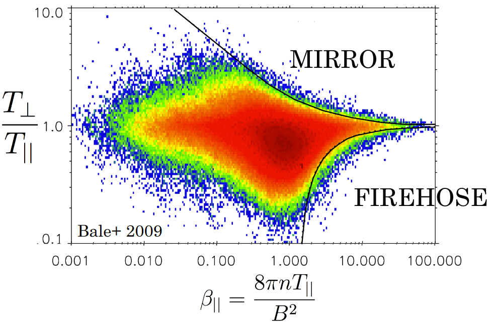
\(\gamma\propto k_\parallel\) leads to UV catastrophe: within KMHD (\(\omega\ll\Omega_i, kr_i\ll 1\)), the wavenumber of peak \(\gamma\) is not captured. Including finite larmor radius gives (Oxford MNRAS 405, 291? ARE THE EXPRESSIONS CORRECT?) \[ \begin{aligned} \gamma_{\text{peak}}\sim \bigg\lvert A + \frac{2}{\beta_\parallel} \bigg\rvert \Omega_i \\ k_{\parallel\text{peak}}r_i\sim \bigg\lvert A + \frac{2}{\beta_\parallel} \bigg\rvert^{1/2} \end{aligned} \] so the instability is very fast (\(\gamma \propto \Omega_i\) very large with strong B field) at microscale. Any high-\(\beta\) macroscopic solution with \(p_\parallel > p_\perp\) will blow up instantly. What happens next is decided by the nonlinear saturation of the firehose. It was a transformative moment when Justin Kasper in 2002 discovered that the firehose stability boundary constrains most observed solar wind states, followed by Hellinger in 2006. Bale in 2009 showed that there is an increased fluctuation level at the boundary.
ADD FIGURE ABOUT THE FIREHOSE STABILITY REGIME FIGURE!
14.2 Mirror Instability: Linear Theory
Let us go back to Equation 14.13 and Equation 14.14 and get apart from Alfvénic what other perturbations there are and when they are stable. We have already looked at the Alfvénic perturbation \(\delta\hat{b}=\delta \mathbf{B}_\perp/B\). Now consider \[ \frac{\delta B}{B} = \frac{\delta B_\parallel}{B} \tag{14.17}\]
From Equation 14.13, we have the perpendicular compression increases B: \[ \omega\frac{\delta B}{B} = \mathbf{k}_\perp\cdot\delta\mathbf{u}_\perp \]
Take \(\mathbf{k}_\perp\cdot\) Equation 14.14: \[ \omega\rho\mathbf{k}_\perp\cdot\delta\mathbf{u}_\perp = \rho\omega^2 \frac{\delta B}{B} = k_\perp^2\Big( \delta p_\perp + \frac{B\delta B}{\mu_0} \Big) + k_\parallel^2\Big( p_\perp - p_\parallel + \frac{B^2}{\mu_0} \Big) \frac{\delta B}{B} \tag{14.18}\]
Note the \(p_\perp\) term here: we need kinetic theory to calculate this! Fortunately we have Equation 14.12 ready for calculating \[ \delta p_\perp = \int \mathrm{d}\mathbf{w}\frac{m_sw_\perp^2}{2}\delta f_s(w_\perp, w_\parallel) \]
\(\delta f_s(w_\perp, w_\parallel)\) can be obtained by calculating \(F_s(\mu,\epsilon)\) and transforming back to \(w_\perp,w_\parallel\).
Here is a cute subtlety: our macroscopic equilibrium, around which we are expanding the distribution is \[ F_{0s}(\mu,\epsilon) = f_{0s}(w_\perp,w_\parallel) = f_{0s}\Big( \sqrt{\frac{2B_0\mu}{m_s}},\sqrt{\frac{2(\epsilon-\mu B_0)}{m_s}} \Big) \] which contains \(B_0\) the unperturbed magnetic field. \(\mu\) in \(F_0\) contains \(B_0+\delta B\), and this has to be taken into account when transforming to \(w_\perp,w_\parallel\). Now when we perturb everything: \[ \begin{aligned} F_s(\mu,\epsilon) &= F_{0s}(\mu,\epsilon) + \delta F_s \\ &= f_{0s}(w_\perp,w_\parallel) + \delta f_s \\ &= f_{0s}\Big( \sqrt{\frac{2\mu(B_0+\delta B)}{m_s}},\sqrt{\frac{2[\epsilon-\mu(B_0+\delta B)]}{m_s}} \Big) + \delta f_s \\ &= f_{0s}\Big( \sqrt{\frac{2\mu B_0}{m_s}}\sqrt{1+\frac{\delta B}{B_0}},\sqrt{\frac{2(\epsilon-\mu B_0)}{m_s}}\sqrt{1-\frac{m_s\mu\delta B}{(\epsilon-\mu B_0)}} \Big) + \delta f_s \\ &\approx f_{0s}\Big( \sqrt{\frac{2\mu B_0}{m_s}},\sqrt{\frac{2(\epsilon-\mu B_0)}{m_s}} \Big) + \frac{2\mu}{m_s}\delta B\Big(\frac{\partial f_{0s}}{\partial w_\perp^2}-\frac{\partial f_{0s}}{\partial w_\parallel^2} \Big) + \delta f_s \end{aligned} \]
Thus \[ \delta f_s = \delta F_s - w_\perp^2\frac{\delta B}{B}\Big(\frac{\partial f_{0s}}{\partial w_\perp^2}-\frac{\partial f_{0s}}{\partial w_\parallel^2} \Big) \]
If \(f_{0s}\) is a bi-Maxwellian, \[ f_{0s} = \frac{n_s}{\pi^{3/2}v_{\text{th}\perp s}^2 v_{\text{th}\parallel s}}\exp\Big(-\frac{w_\perp^2}{v_{\text{th}\perp s}^2}-\frac{w_\parallel^2}{v_{\text{th}\parallel s}^2}\Big) \] then this can be further written as \[ \delta f_s = \delta F_s + w_\perp^2\frac{\delta B}{B}\Big(\frac{1}{v_{\text{th}\perp s}^2} - \frac{1}{v_{\text{th}\parallel s}^2} \Big) f_{0s} = \delta F_s + w_\perp^2\frac{\delta B}{B}\frac{m_sn_s}{2}\Big(\frac{1}{p_{\perp s}} - \frac{1}{p_{\parallel s}} \Big) f_{0s} \]
We can eliminate the partial derivatives via integration by parts: \[ \begin{aligned} \int \mathrm{d}\mathbf{w}\frac{\partial f_{0s}}{\partial w_\parallel^2} &= \int_0^{2\pi}\mathrm{d}\theta \int dw_\perp\int \frac{1}{2w_\parallel}\frac{\partial f_{0s}}{\partial w_\parallel}dw_\parallel \\ &= \int_0^{2\pi}\mathrm{d}\theta \int dw_\perp\int\frac{1}{2w_\parallel}\mathrm{d} f_{0s} \\ &= \int_0^{2\pi}\mathrm{d}\theta \int dw_\perp\Big[\cancel{\frac{f_{0s}}{2w_\parallel}\bigg\rvert_{-\infty}^{\infty}} - \int f_{0s}\mathrm{d}\frac{1}{2w_\parallel}\Big] \\ &= \int_0^{2\pi}\mathrm{d}\theta \int dw_\perp\int\frac{1}{2w_\parallel^2}f_{0s}dw_\parallel \\ &= \int \mathrm{d}\mathbf{w} \frac{1}{2w_\parallel^2}f_{0s} \\ \int \mathrm{d}\mathbf{w}w_\perp w_\perp^4\frac{\partial f_{0s}}{\partial w_\perp^2} &= 2\pi\int dw_\parallel \Big[ \cancel{\frac{1}{2}w_\perp^4f_{0s}\bigg\rvert_{-\infty}^{+\infty}} - \frac{1}{2}\int f_{0s}dw_\perp^4 \Big] \\ &= -2\pi\int dw_\parallel 2w_\perp^2 f_{0s}w_\perp dw_\perp \\ &= -2 \int \mathrm{d}\mathbf{w} w_\perp^2 f_{0s} \end{aligned} \]
This then gives us \[ \begin{aligned} \delta p_{\perp s} &= \int \mathrm{d}\mathbf{w}\frac{m_s w_\perp^2}{2}\delta f_s \\ &= \int \mathrm{d}\mathbf{w}\frac{m_s w_\perp^2}{2}\delta F_s - \int \mathrm{d}\mathbf{w}\frac{m_s w_\perp^4}{2}\Big(\frac{\partial f_{0s}}{\partial w_\perp^2}-\frac{\partial f_{0s}}{\partial w_\parallel^2} \Big)\frac{\delta B}{B} \\ &= \int \mathrm{d}\mathbf{w}\frac{m_s w_\perp^2}{2}\delta F_s - \int_0^{2\pi}\mathrm{d}\theta \int dw_\perp w_\perp \int \mathrm{d} w_\parallel \frac{m_s w_\perp^4}{2}\Big(\frac{\partial f_{0s}}{\partial w_\perp^2}-\frac{\partial f_{0s}}{\partial w_\parallel^2} \Big)\frac{\delta B}{B} \\ &= \int \mathrm{d}\mathbf{w}\frac{m_s w_\perp^2}{2}\delta F_s + 2\int \mathrm{d}\mathbf{w}\frac{m_s w_\perp^2}{2}\delta f_{0s}\frac{\delta B}{B} + \int \mathrm{d}\mathbf{w}\frac{2(\frac{1}{2}m_sw_\perp^2)^2}{m_sw_\parallel^2}f_{0s}\frac{\delta B}{B} \\ &= \int \mathrm{d}\mathbf{w}\frac{m_s w_\perp^2}{2}\delta F_s + \frac{\delta B}{B}\Big( 2p_{\perp s} - \frac{2 p_{\perp s}^2}{p_{\parallel s}} \alpha_s ) \end{aligned} \tag{14.19}\] where \(\alpha_s\) is some coefficients of order 1 if \(f_{0s}\) is not bi-Maxwellian.
\(\delta F_s\) can be obtained by ignoring collisions and linearizing and Fourier-transforming Equation 14.12 (\(\mathbf{u}_s=0\)): \[ \begin{aligned} -i(\omega - k_\parallel w_\parallel)\delta F_s = - \Big[ m_sw_\parallel\Big( \frac{q_s}{m_s}E_\parallel - i(\omega-k_\parallel w_\parallel) \delta u_{\parallel s}\Big) -i\omega\mu\delta B \Big]\frac{\partial F_{0s}}{\partial \epsilon} \\ \delta F_s = -i\frac{w_\parallel q_s E_\parallel}{\omega-k_\parallel w_\parallel}\frac{\partial F_{0s}}{\partial \epsilon} - \delta u_{\parallel s}m_sw_\parallel\frac{\partial F_{0s}}{\partial\epsilon} - \frac{\omega}{\omega-k_\parallel w_\parallel}\mu\delta B\frac{\partial F_{0s}}{\partial\epsilon} \end{aligned} \]
The first term can be ignored if \(\beta\gg 1\) (??? See the complete calculation in another note!); otherwise \(E_\parallel\) can be got by imposing \(\sum_s q_s n_s = 0\). The second term can be shown to be equivalent to \(\delta u_{\parallel s}\partial f_{0s}/\partial w_\parallel\): \[ \begin{aligned} \frac{\partial f_{0s}}{\partial w_\parallel} &= \frac{\partial f_{0s}}{\partial \epsilon}\frac{\partial \epsilon}{\partial w_\parallel} + \frac{\partial f_{0s}}{\partial\mu}\cancel{\frac{\partial \mu}{\partial w_\parallel}} \\ &= \frac{\partial F_{0s}}{\partial\epsilon}m_s w_\parallel \end{aligned} \] so this will not contribute to \(\delta p_\perp\) because it integrates to 0.
The third term can be written as \[ \frac{\omega}{\omega-k_\parallel w_\parallel}\mu\delta B\frac{\partial F_{0s}}{\partial\epsilon} = \frac{\omega}{\omega-k_\parallel w_\parallel}\frac{m_sw_\perp^2}{2}\frac{\delta B}{B}\frac{1}{w_\parallel}\frac{\partial f_{0s}}{\partial w_\parallel} = \frac{\omega}{\omega-k_\parallel w_\parallel} m_sw_\perp^2\frac{\delta B}{B}\frac{\partial f_{0s}}{\partial w_\parallel^2} \]
Thus, the “relevant” part of \(\delta F_s\) is \[ \delta F_s = -\frac{\omega}{\omega-k_\parallel w_\parallel} m_sw_\perp^2\frac{\delta B}{B}\frac{\partial f_{0s}}{\partial w_\parallel^2} \] and its contribution to \(\delta p_{\perp s}\) is \[ \int \mathrm{d}\mathbf{w}\frac{m_sw_\perp^2}{2}\delta F_s = \frac{\delta B}{B}\frac{\omega}{|k_\parallel|}\int\frac{dw_\parallel}{w_\parallel - \frac{\omega}{|k_\parallel|}} \Big[ \frac{\partial}{\partial w_\parallel^2}\int \mathrm{d}\mathbf{w}_\perp \frac{m_s^2w_\perp^4}{2} f_{0s} \Big] \]
Here we have \(|k_\parallel|\) because if \(k_\parallel <0\), we can change the variable \(w_\parallel \rightarrow -w_\parallel\). This involves the Landau integral, which can be evaluated with the residual theorem Equation 3.11 when integrate in the complex plane mostly along the real axis and the large semicircle in the upper half plane except for a small semicircle just below the pole (ADD FIGURE!): \[ \frac{1}{w_\parallel - \frac{\omega}{|k_\parallel|}} = P\frac{1}{w_\parallel - \frac{\omega}{|k_\parallel|}} + i\pi\delta\Big(w_\parallel - \frac{\omega}{|k_\parallel|} \Big) \] so \[ \begin{aligned} \int \mathrm{d}\mathbf{w}\frac{m_sw_\perp^2}{2}\delta F_s &= \frac{\delta B}{B}\Big[ \cancel{\frac{\omega}{|k_\parallel|}P\int\frac{dw_\parallel}{w_\parallel - \frac{\omega}{|k_\parallel|}} \big[ ... \big]} + i\pi\frac{\omega}{|k_\parallel|}\big[ ... \big]_{w_\parallel}=\omega/|k_\parallel| \Big] \end{aligned} \]
The first term is small when we assume \(\omega\ll k_\parallel v_{\text{th}s\parallel}\); the second term must be kept because it is the lowest-order imaginary part which will lead to instability.
For a bi-Maxwellian, \[ \Big[ \frac{\partial}{\partial w_\parallel^2}\int \mathrm{d}\mathbf{w}_\perp\frac{m_s^2w_\perp^4}{2}f_{0s} \Big]_{w_\parallel=\omega/|k_\parallel|} = -\frac{2p_{\perp s}^2}{p_{\parallel s}}\frac{e^{-\frac{\omega^2}{k_\parallel^2 v_{\text{th}\parallel s}^2}}}{\sqrt{\pi}v_{\text{th}\parallel s}} \]
The exponential term is nearly 1. If it is not a bi-Maxwellian, then we need to multiply by a coefficient \(\alpha_s \sim 1\).
Equation 14.19 becomes \[ \delta p_{\perp s} = \frac{\delta B}{B}\Big[ 2p_{\perp s} - \frac{2p_{\perp s}^2}{p_{\parallel s}}\Big( \alpha_s + i\sqrt{\pi}\frac{\omega}{|k_\parallel|v_{\text{th}\parallel s}}\sigma_s \Big) \Big] \]
This goes into Equation 14.18: \[ \rho \omega^2 = k_\perp^2\frac{B^2}{\mu_0}\Big[ \sum_s(1 - \frac{p_{\perp s}}{p_{\parallel s}}\alpha_s)\beta_{\perp s} - i\sum_s \sigma_s\frac{p_{\perp s}}{p_{\parallel s}}\beta_{\perp s}\sqrt{\pi}\frac{\omega}{|k_\parallel| v_{\text{th} \parallel s}} + 1 \Big] + k_\parallel^2 \frac{B^2}{\mu_0}\Big[ \sum_s\frac{\beta_{\perp s}}{2}\big( 1 - \frac{p_{\parallel s}}{p_{\perp s}} \big) + 1 \Big] \]
The left-hand side can be neglected because \(\omega\ll k_\parallel v_{\text{th}\parallel s}\). The electron thermal velocity \(v_{\text{th}\parallel e}\) in the denominator can be neglected because \(v_{\text{th}\parallel e} \gg v_{\text{th}\parallel i}\). The growth rate \(\gamma\) is the imaginary part of \(\omega\). Reorganize the last equation: \[ \sigma_i\frac{p_{\perp i}}{p_{\parallel i}}\beta_{\perp i}\sqrt{\pi}\frac{\gamma}{|k_\parallel|v_{\text{th}\parallel i}} = \sum_s \Big(\frac{p_\perp s}{p_\parallel s}\alpha_s - 1 \Big)\beta_{\perp s} - 1 -\frac{k_\parallel^2}{k_\perp^2}\Big[ \sum_s\frac{\beta_{\perp s}}{2}\big( 1-\frac{p_{\parallel s}}{p_{\perp s}}\big) + 1 \Big] \tag{14.20}\] where \(\Lambda\equiv \frac{k_\parallel^2}{k_\perp^2}\sum_s \Big(\frac{p_\perp s}{p_\parallel s}\alpha_s - 1 \Big)\beta_{\perp s} - 1\) triggers instability if this is positive: \[ \sum_s \Big(\frac{p_\perp s}{p_\parallel s}\alpha_s - 1 \Big)\beta_{\perp s} > 1 \]
Examining where this comes from, we see that this amounts to \(\delta p_\perp\) modifying the magnetic pressure force and turning it from positive to negative: \[ \delta p_\perp + \frac{B\delta B}{\mu_0} = \frac{B\delta B}{\mu_0}\Big[ \underbrace{1}_{\text{B pressure}} - \underbrace{\sum_s\Big( \frac{p_{\perp s}}{p_{\parallel s}}\alpha_s - 1 \Big)\beta_{\perp s}}_{\substack{\text{non-resonant} \\ \text{particle pressure}}} + \underbrace{...}_{\substack{\text{resonant particle} \\ \text{pressure}}} \Big] \]
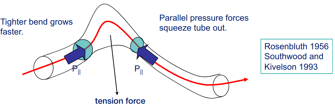
Thus, fundamentally, pressure anisotropy makes it easier to compress or rarefy magnetic field — and things become unstable when the sign of the pressure flips and it becomes energetically profitable to create compressions and rarefications. (ADD FIGURE!) The dispersion relation Equation 14.20 is basically a statement of pressure balance between the magnetic pressure, the non-resonant particle pressure \(\delta p_\perp\) and the resonant particle pressure \(\propto\gamma\), which came from the betatron acceleration \(\mu \mathrm{d}B/\mathrm{d}t\) in Equation 14.12. (See also Eq. 21 in Southwood and Kivelson (1993))
The betatron acceleration term refers to what happens in the stable case. When magnetic pressure opposes formation of \(\delta B\) perturbations (say, troughs), to compensate it, we must have \(\gamma<0\) and energy goes from \(\delta B\) to resonant particles, which are accelerated by the mirror force. The corresponding decaying of \(\delta B\) is the well-known Barnes damping.1
More discussion on the physics is presented by Southwood and Kivelson (1993). They pointed out that although the instability is resonant, the role of resonant particle is unusual. The instability results from pressure imbalance between the bulk of the plasma and the magnetic field. For this to occur, the bulk (nonresonant) pressure response must be in antiphase with the magnetic pressure as occurs at low frequencies when the magnetic moment and the particle energy are conserved. The resonant particles produce a pressure perturbation, however, in phase with the field pressure change. A corollary is that unlike the nonresonant particles,the resonant particles experience energy changes as the instability develops. The linear growth rate of most resonant instabilities is proportional to the number of resonant particles. However, in the case of the mirror instability, the growth is inversely proportional to the number (and pressure contribution) of resonant particles.The reason for the anomalous result is that the fewer particles there are at small parallel velocity the higher the growth rate needs to be to balance the pressure imbalance generated by the nonresonant distribution.
To finish the job, note that, from Equation 14.20 (ADD FIGURE!) for a given \(k_\perp\) \[ \frac{\partial\gamma}{\partial k_\parallel}\bigg\rvert_{k_\perp} \propto \Lambda - \frac{k_\parallel^2}{k_\perp^2}\Big[\sum_s\frac{\beta_{\perp s}}{2}\Big(1-\frac{p_\parallel s}{p_\perp s} \Big) + 1 \Big] \]
The maximum growth rate is reached when the right-hand side goes to 0, which is equivalent to \(\frac{2}{3}\Lambda\), so the maximum growth rate \[ \gamma_{\text{max}} = \frac{|k_\parallel|v_{\text{th}\parallel i}}{\sqrt{\pi}}\frac{2}{3}\Lambda \frac{p_{\parallel i}}{p_{\perp i}}\frac{1}{\sigma_i\beta_{\perp i}} \]
We have assumed \(\gamma\ll k_\parallel v_{\text{th}\parallel s}\), which is indeed true if \[ \Lambda\frac{1}{\beta_{\perp i}} = \big(\sum_s A_s \beta_{\perp s} - 1 \big)\frac{1}{\beta_{\perp i}}\ll 1 \] so our approximations are consistent.
If we are close to marginal instablity, \[ \frac{k_\parallel}{k_\perp}\sim\sqrt{\Lambda}\ll 1 \] so mirror modes are highly oblique near the threshold.
Another important point is that again we encounter the UV catastrophe since \(\gamma\propto k_\parallel\). The mirror mode is a fast, microscale instability whose peak growth rate is outside KMHD regime. Including finite larmor radius gives (Hellinger 2007 PoP 14, 082105?) \[ \gamma_{\text{peak}}\sim\Big(A-\frac{1}{\beta}\Big)^2\beta\Omega_i,\quad k_{\text{peak}}r_i\sim\Big( A-\frac{1}{\beta}\Big)\beta \]
Thus, any high-\(\beta\) macroscopic solution of KMHD with \(p_\perp>p_\parallel\) will blow up, just like the case for \(p_\parallel > p_\perp\), and again what happens next depends on how mirror instability saturates. Note that \(A_e\) is ignored since \(A_e\ll A_i\) (?). The mirror instability condition is \[ \begin{aligned} \frac{p_{\perp i}}{p_{\parallel i}} - 1 > \frac{1}{\beta_{\perp i}} = \frac{1}{\beta_{\parallel i}}\frac{p_{\parallel i}}{p_{\perp i}} \\ \frac{p_{\perp i}}{p_{\parallel i}}\Big( \frac{p_{\perp i}}{p_{\parallel i}}-1\Big) > \frac{1}{\beta_{\parallel i}} \end{aligned} \]
Figure 14.2 shows observation from Wind spacecraft. The solar wind indeed seems to stay within these boundaries. (ADD REFS!)
14.2.1 Comparison With Slow Mode
- Driving Mechanism
- Mirror Mode: Driven primarily by pressure anisotropy (\(T_\perp/T_\parallel > 1\)) in high-beta plasmas.
- MHD Slow Mode: Driven by pressure gradients and magnetic field line curvature in low- to moderate-beta plasmas.
- Propagation Characteristics
- Mirror Mode: Primarily propagates parallel to the background magnetic field, but can have a small perpendicular component. It is a non-propagating mode in the fluid limit (zero frequency), but it can acquire a finite frequency due to kinetic effects.
- MHD Slow Mode: Propagates obliquely to the magnetic field, with both parallel and perpendicular components. It is a propagating mode with a finite frequency.
- Plasma Conditions
- Mirror Mode: Typically found in high-beta (\(\gtrsim 1\)) plasmas, such as the Earth’s magnetosheath and the solar wind.
- MHD Slow Mode: More common in low- to moderate-beta (\(\ll 1\)) plasmas, such as the solar corona and the Earth’s magnetosphere, where the magnetic pressure dominates.
14.3 Origin of Pressure Anisotropy
So far we have seen that the bottom line is that any macroscopic, high-\(\beta\) KMHD solution that has \(p_\perp\neq p_\parallel\) (more precisely, \(|p_\perp - p_\parallel|/p \gtrsim 1/\beta\)) will be voilently unstable to either firehose or mirror — both of which are fast and micro-scale modes giving rise to fluctuations outside the KMHD regime (and, by the way, also outside gyrokinetics — too close to cyclotron frequency, \(k_\parallel/k_\perp\) not small enough, \(\delta\mathbf{B}/B\) also not small enough). How worried should this make us about the applicability of KMHD to high-\(\beta\) plasmas that are not collisional enough to be fully fluid (i.e. \(\nu\ll\Omega_s\))?
The answer is, very worried! A key property of low-frequency, weakly collisional dynamics is that the magnetic moment \(\mu=m_sw_\perp^2/2B\) is conserved by particles. The mean \(\mu\) of particles of species \(s\) is \[ <\mu>_w = \frac{1}{n_s}\int \mathrm{d}\mathbf{w}\mu f_s = \frac{p_{\perp s}}{n_s B} = \text{const.} \]
For the purpose of a qualitative discussion, let us pretend for a moment that \(n_s=\text{const}\) (incompressible plasmas, \(\beta\gg 1\)). Then the above conservation relation says that, locally in a fluid element (\(\mathbf{w}\) is peculari velocity), every time you change \(\mathbf{B}\), you must change \(p_{\perp s}\) proportionally (but not \(p_{\parallel s}\)). Thus we expect (?) \[ \frac{1}{p_{\perp s}}\frac{\mathrm{d} p_{\perp s}}{\mathrm{d}t}\sim\underbrace{\frac{1}{B}\frac{\mathrm{d}B}{\mathrm{d}t}}_{\mu\text{ conservation}} - \underbrace{\nu_s\frac{p_{\perp s}-p_{\parallel s}}{p_{\perp s}}}_{\substack{\text{relaxation of pressure} \\ \text{anisotropy by collisions}}} \tag{14.21}\]
It is useful to remind ourselves that \(\mathrm{d}/\mathrm{d}t\) is in the \(\mathbf{u}_s\) frame. Balancing the two effects on the right-hand side, \[ \Delta_s = \frac{p_{\perp s} - p_{\parallel s}}{p_{\perp s}} \sim\frac{1}{\nu_s}\frac{1}{B}\frac{\mathrm{d}B}{\mathrm{d}t} \tag{14.22}\]
This expression is valid only if \(\Delta_s\ll 1\), i.e. \(\nu_s\gg \frac{1}{B}\frac{\mathrm{d}B}{\mathrm{d}t}\), otherwise \(\Delta_s\) will grow with time as B is changed. Thus
- B increases locally \(\rightarrow \Delta_s >0 \rightarrow\) mirror
- B decreases locally \(\rightarrow \Delta_s <0 \rightarrow\) firehose
As nealy any large-scale dynamics involves local changes in \(\mathbf{B}\), this means that nearly any macroscopic solution of KMHD in the high-\(\beta\) regime will be unstable. A very good example is the dynamo problem: when magnetic field is randomly stretched by turbulence, leading (in MHD) to exponential growth of magnetic energy (and, eventually, to saturated fields we observe), locally one find structures of this sort: (ADD FIGURE!)
Generally speaking, in order to understand long-time evolution, we need some sort of mean-field theory for the large-scale effect of the microscale instabilities on the dynamics. Presumably, this is to keep preserve anisotropy, marginal out (?) the instabilities (as indeed appears to be confirmed by the solar wind measurements — see Bale + 2009).
There are two ways in which this can happen — firehose and mirror fluctuations might scatter particles, leading to higher effective collisionality and ? control the pressure anisotropy \[ -\frac{2}{\beta}\lesssim \frac{p_\perp - p_\parallel}{p}\lesssim \frac{1}{\beta} \]
They might inhibit changes of B, which is another way of keeping \(\Delta\) under control. Which of these matters for dynamics, see the speculative overview of the possible consequences of either mechanisim in MNRAS 440, 3226 (2014).
- nonlinear firehose: Rosin+ MNRAS 413 2011
- nonlinear mirror: Rincon+ MNRAS 447, 2015
- PIC simulations: Kunz+ PRL, 2014
14.4 Remarks
14.4.1 Remark I
If we assume incompressibility, the magnetic induction Equation 14.7 becomes \[ \begin{aligned} \frac{\mathrm{d}\mathbf{B}}{\mathrm{d}t} = \mathbf{B}\cdot\nabla\mathbf{u} \\ \frac{1}{B}\frac{\mathrm{d}B}{\mathrm{d}t} = \hat{b}\hat{b}:\nabla\mathbf{u} \end{aligned} \]
Then, from Equation 14.22, \[ p_{\perp s} - p_{\parallel s}\sim\frac{p_s}{\nu_c}\hat{b}\hat{b}:\nabla\mathbf{u} \] where \(p_s/\nu_c\) is the parallel dynamical viscosity. Putting this back into Equation 14.10, we get the lowest order ??? MHD equation. So, from the large-scale point of view, pressure anisotropy is viscous stress — but the resulting equations are ill-posed (blow up via instabilities with \(\gamma\propto k_\parallel\)).
14.4.2 Remark II
More rigorously, Equation 14.21 can be obtained via “CGL equations”, i.e. the evolution equations of \(p_{\perp s}\) and \(p_{\parallel s}\). Namely \(\int \mathrm{d}\mathbf{w}\frac{m_sw_\perp^2}{2}\) Equation 14.11: \[ p_{\perp s}\frac{\mathrm{d}}{\mathrm{d}t}\ln\frac{p_{\perp s}}{n_s B} = -\nabla\cdot(q_{\perp s}\hat{b}) - q_{\perp s}\nabla\cdot\hat{b} - \nu_s(p_{\perp s} - p_{\parallel s}) \tag{14.23}\]
\(\int \mathrm{d}\mathbf{w}m_sw_\parallel^2\) Equation 14.11: \[ p_{\parallel s}\frac{\mathrm{d}}{\mathrm{d}t}\ln\frac{p_{\parallel s}B^2}{n_s^3} = -\nabla\cdot(q_{\parallel s}\hat{b}) + 2q_{\perp s}\nabla\cdot\hat{b} - 2\nu_s (p_{\parallel s} - p_{\perp s}) \tag{14.24}\]
The left-hand side is the conservation of \(J=\oint dl w_\parallel\), i.e. “bounce invariant”. The new feature here is heat fluxes: \[ \begin{aligned} q_{\perp s} = \int \mathrm{d}\mathbf{w}\frac{m_sw_\perp^2}{2}w_\parallel f_s \\ q_{\parallel s} = \int \mathrm{d}\mathbf{w}m_sw_\parallel^3 f_s \end{aligned} \]
They are here because particles can flow in and out of a fluid element and thus affect the conservation (or otherwise) of \(<\mu>_w\) and \(<J^2>_w\) within it.
Finally, from Equation 14.23 and Equation 14.24, \[ \begin{aligned} \frac{\mathrm{d}}{\mathrm{d}t}(p_{\perp s} - p_{\parallel s}) &= (p_{\perp s} + 2p_{\parallel s})\frac{1}{B}\frac{\mathrm{d}B}{\mathrm{d}t} + (p_{\perp s} - 3p_{\parallel s})\frac{1}{n_s}\frac{dn_s}{\mathrm{d}t} \\ &-\nabla\cdot[(q_{\perp s}-q_{\parallel s})\hat{b}] - 3q_{\perp s}\nabla\cdot\hat{b} - 3\nu_s(p_{\perp s} - p_{\parallel s}) \end{aligned} \]
???
\[ \begin{aligned} \Delta_s &= \frac{p_{\perp s}-p_{\parallel s}}{p_s} \\ &\approx \frac{1}{\nu_s}\Big\{ \frac{1}{B}\frac{\mathrm{d}B}{\mathrm{d}t} - \frac{2}{3}\frac{1}{n_s}\frac{dn_s}{\mathrm{d}t} - \frac{\nabla\cdot[((q_{\perp s} - q_{\parallel s})\hat{b})] + 3q_{\perp s}\nabla\cdot\hat{b}}{3p_s} \Big\} \end{aligned} \]
Typically, what prominent here are electron heat fluxes. So heat fluxes can also lead to anisotropies and so macroscopic solutions of KMHD involving temperature gradients will also go unstable at microscales!
So here we are, we cannot change B at large scales, we cannot compress/rarefy the plasma and we cannot have temperature gradients without having to deal everything exploding and needing new equations. Enjoy!
Landau damping of “mirror field”, Barnes 1966, also known as transit-time damping from Stix’s book.↩︎