25 Aurora
The aurora is a visible and fascinating consequence of the complex magnetospheric processes that are driven by the interaction between the solar wind and the geomagnetic field. The aurora can appear as a diffuse plae band crossing the sky from east to west, or as rapidly moving bright and colorful curtains and rays covering a large fraction of the sky. We will not attempt to describe all the various forms that auroras may appear in, but only distinguish between diffuse and discrete auroras. The particles that cause these two main types are precipitated into the atmosphere by rather different physical processes. Magnetospheric substorms and the mechanisms leading to the formation of discrete auroras are still at the frontier of magnetospheric research. This chapter is mostly based on Chapter 10 in the lecture notes of Prof. Kjell Rönnmark.
25.1 Auroral Light Emission
There are numerous ancient legends and beliefs about the aurora from various parts of the world. Many of the mythological ideas, as well as more scientific theories from the eighteenth century, explained the aurora as sunlight reflected, refracted, or scattered by various divine or natural processes. Observations reveal that it consists of discrete spectral lines, which proves that auroral light is emitted by a gas, and rules out reflected or scattered sunlight. The strongest line the auroral spectrum is found to be \(557.7\,\mathrm{nm}\).
Auroras are caused by charged particles with energy in the range from 10 eV to 30 keV. These particles collide in the upper atomosphere with atoms and molecules that are left in an excited state after the collision. About 90% of the aurora is caused by electrons, and the rest by protons. At altitudes about 100 km where most of the auroral light is emitted, the atmosphere consists mainly of nitrogen and oxygen as shown in Fig. ???. In these gases the quantum mechanically allowed transitions that produce strong spectral lins are all outside the visible part of the spectrum — otherwise air would not be transparent and colourless. The visible auroral emissions are due to transitions from forbidden metastable states, with low transition probabilities and long lifetimes. If the gas pressure is too high, these metastable states will relax to the ground state through collisions long before they decay by emitting light. However, at altitudes above 100 km collisions are sufficiently rare to allow the decay of an excited state of atomic oxygen. This state has an excitation energy of 4.17 eV and a lifetime of 0.8 s. It decays in a two step process. The green line is emitted in the first step, which takes the atom to a state at 1.96 eV. This intermediate state has a very long lifetime, 110 s, and the the red line emission at 630.0 nm that takes it to the ground state mainly occurs at altitudes above 200 km. This red line can also be produced by direct excitation to the state at 1.96 eV by collisions with low energy electrons. Other strong lines in the auroral spectrum are emitted by nitrogen. Molecular \(\mathrm{N}_2^+\) ions are created in an excited state by collisions, and they decay to their ground state by emitting a bluish-voilet line at 427.8 nm. Sometimes the lowest part of strong auroras are colored red by emissions near 600 nm from neutral \(\mathrm{N}_2\) molecules.
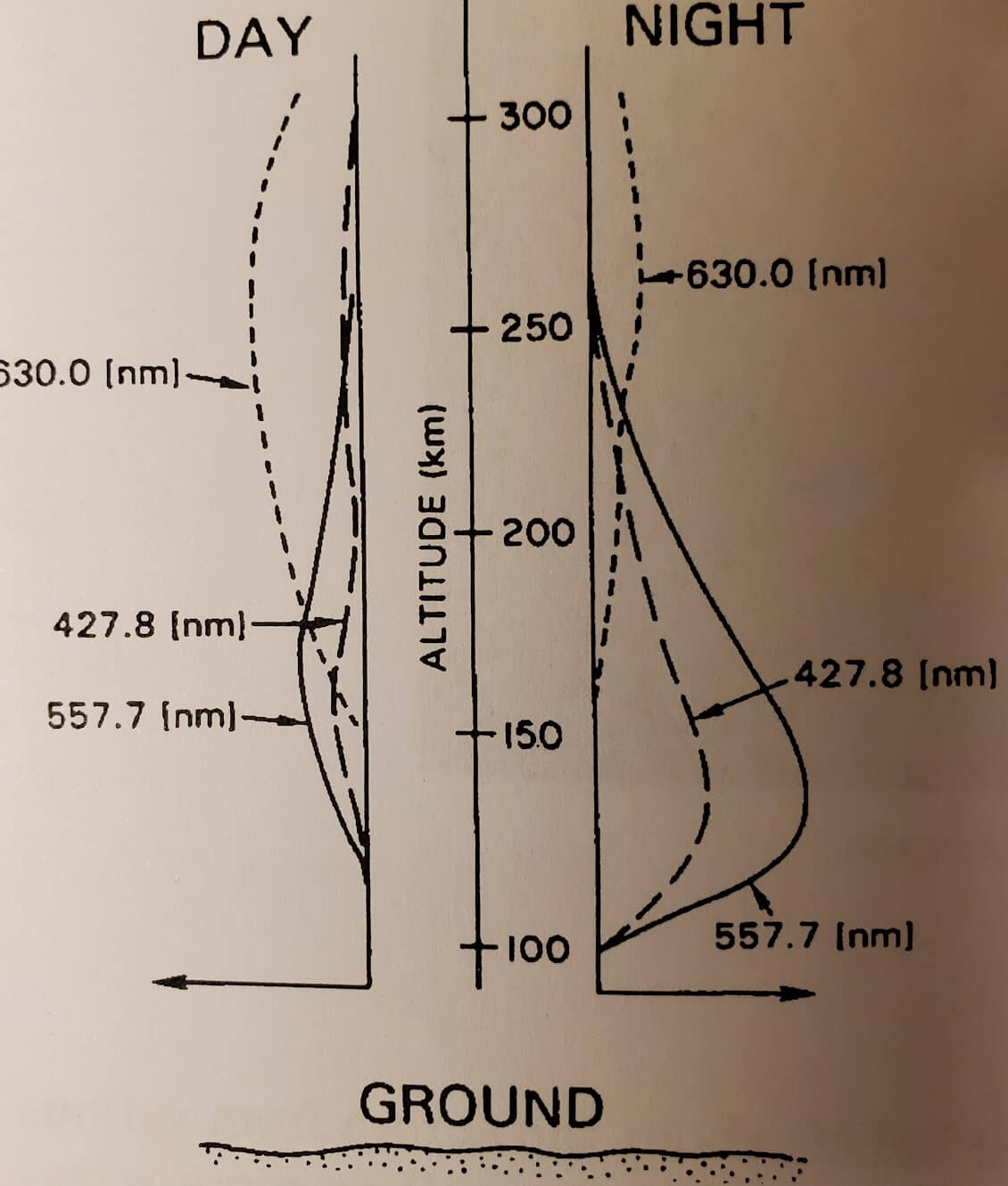
Figure 25.1 shows the typical altitude distribution of the auroral emissions. The cross section for excitation of the different lines depends on the energy of the incoming auroral particles. Usually, the precipitating particles have higher energy at night than during the day. Low energy electrons give up their energy at higher altitudes, and produces more red emissions. Another difference between day and night is that resonant scattering by sunlight enhances the \(\mathrm{N}_2^+\) line 427.8 nm relative to the green line.
25.2 Diffuse Aurora
Some diffuse aurora is nearly always found in the auroral zone. On a clear and dark night it is often seen as a diffuse band, which may appear gray if the intensity is below the color threshold of the eye. Even if no aurora can be seen from the ground, we know from satellite observations of precipitating particles and auroral spectral lines in the UV-range that the diffuse aurora forms a rather continuous band aroud the auroral zone.
Magnetosheath particles that enter through the magnetopause cusps are a source of diffuse aurora on the dayside. In the cusps there are field lines that connect the ionosphere to the magnetosheath, and magnetosheath particles with sufficiently small pitch angles will precipitate along these field lines. Around local noon, there will be a continuous flux of low energy (\(\le 100\,\mathrm{eV}\)) particles, which at altitudes above 200 km cause a diffuse band of emissions at 630 nm.
On the nightside, and far into the evening and morning, diffuse auroras are caused by particles of plasmasheet origin. The energy spectrum of these particles extends from below 100 eV to above 20 keV. The continuous precipitation of electrons from the plasmasheet presents a problem, which has not been completely solved yet. Most of the plasmasheet is on closed field lines, and the loss cone in a stationary magnetosphere should be empty (because particles will be lost). To explain the diffuse aurora, we need some mechanisms that can scatter the particles into the loss cone.
Plasma waves in the equatorial magnetosphere can cause strong pitch-angle scattering if they are resonant with the particles. Resonant in this context means that the parallel velocity of the particle and the phase velocity of the wave are related so that the particle feels an electric field that oscillates at the gyrofrequency. Significant changes in the velocities of the particles occur since they systematically gain or lose energy while they are resonant. At least for electrons with energy higher than a few keV, the required pitch-angle scattering can be provided by a type of waves in the whistler mode, known as magnetospheric hiss. However, the phase velocity of whistler mode waves may be too high to give resonance with lower energy electrons. Low energy electrons can be scattered efficiently by waves in the upper hybrid mode. Upper hybrid waves are electrostatic waves, but it is not clear that these waves are sufficiently common to explain the diffuse precipitation of low energy electrons.
25.3 Auroral Waves and Ion Heating
Plasma waves play several roles on the auroral stage. As we have seen, waves near the equator provide the pitch angle scattering that causes diffuse aurora. Closer to Earth there are several types of plasma waves that are generated by the intense flux of particles precipitating into the aurora.
Discrete auroras are strong sources of whistler modes that appear rather different from whistlers generated by lightning. The auroral emissions are characterized by a broadband spectrum covering frequencies from a few kHz to hundreds of kHz, and they are continously generated with only slow amplitude variations. If the signal is amplified and connected to a loudspeaker a hissing noise is heard, and these waves are called auroral hiss. The auroral hiss propagates from the upper ionosphere to the equatorial magnetosphere where it contributes to the magnetospheric hiss. Auroral hiss also propagates to the ground, and at auroral latitudes it will cause noise in radio receivers tuned to low frequencies.
An interesting wave emission connected to discrete auroral arcs is called Auroral Kilometric Radiation (AKR). This is an intense radio wave radiation with peak intensity at frequencies just below 300 kHz, corresponding to a kilometric wavelength. However, the frequency can vary from 50 kHz to 1 MHz. The AKR is generated by a mechanism involving subtle relativistic effects ina low density plasma at a frequency very close to the local electron gyrofrequency. The highest frequencies are generated cloeet to Earth, where the magnetic field is strongest.The maximum power transmitted as AKR has been estimated to 1 GW, which makes auroras the strongest sources of radio waves from Earth. EM radiation at these frequencies can propagate freely out of the magnetosphere where the density is low, but it will be reflected from the ionosphere at the level where the wave frequency equals \(\omega_{pe}\). Hence, AKR signals cannot be received on the ground, and although these emissions are very strong they were not discovered until 1965. In fact, the corresponding auroral emission from Jupiter, which is known as Jovian decametric radiation and has higher frequency, was observed by radio astronomers ten years earlier.
Electrostatic plasma oscillations and other electrostatic waves are also generated above auroral arcs. Electrostatic waves with low frequencies, in the vicinity of the ion gyrofrequencies, have important effects on the magnetospheric dynamics. These waves are generated by the auroral electrons, but they are damped by the ions. The wave energy absorbed by the ions goes mainly into their perpendicular velocities. The magnetic moment then increases, and the ions are pushed out of the ionosphere by the magnetic mirror force \(\mu\nabla B\). This process can cause a flow of at least \(10^{25}\,O^+\) per second from the auroral ionosphere during times of auroral activity. This flow gives the magnetosphere a significant content of ionospheric particles, and reduces the plasma density in the upper ionosphere above auroral arcs. In the auroral cavity dug out by ion heating the electron density is often about \(3\times10^5\,\mathrm{m}^{-3}\) down to altitudes below \(1\,\mathrm{R}_\mathrm{E}\), at least when the ionosphere is in darkness. This density reduction is essential for the generation of AKR, and as we shall see also for the generation of discrete auroras.
25.4 Substorms and Discrete Aurora
Magnetospheric substorms arise due to an imbalance between the dayside and nightside reconnection rates. As a simple example, this can arise during a sudden rotation of the IMF from northward to southward. A southward IMF leads to an increased reconnection rate at the magnetopause. More plasma and more magnetic flux is then transported to the magnetotail in \(\mathcal{O}(10^2)\,\mathrm{s}\), and the pressure in the tail lobes increases. The plasmasheet is compressed, which on the ground can be seen as an equatorward motion and brightening of a pre-existing diffuse arc. The increased precipitation from the squeezed plasmasheet will also intensify ion heating, which leads to lower densities in the upper ionosphere above the auroral arc. As the density of the cross tail current increases and the neutral sheet becomes thinner, an unstable situation builds up. At this stage, reconnection starts in some part of the tail (Figure 25.2). This marks the onset of a magnetospheric substorm, and the process of storing energy in the magnetotail described above is often called the substorm growth phase.
The original usage of “substorm” comes from Akasofu and Chapman (1961), and was used to describe the short-term magnetic variations during the main phase of a magnetic storm. The current definition did not develop until a decade later, after it became clear that substorms and storms were distinctly different geomagnetic phenomena. The collection of phenomena that includes auroral breakup and expansion, the substorm current wedge, near-Earth dipolarization, and Pi2 pulsations, became collectively known as the magnetospheric substorm.
The concept of the substorm current wedge (SCW) has played an important role in understanding the coupling of the magnetotail to the ionosphere during substorms. It provides a simple explanation for the magnetic perturbations observed at mid and low latitudes during substorms, and is useful in understanding the magnetic variations seen in the auroral zone. In its simplest form, a model of the current wedge consists of a single loop with line currents into and out of the ionosphere on dipole field lines connected by a westward ionospheric line current and by an eastward magnetospheric line current (Figure 25.2).
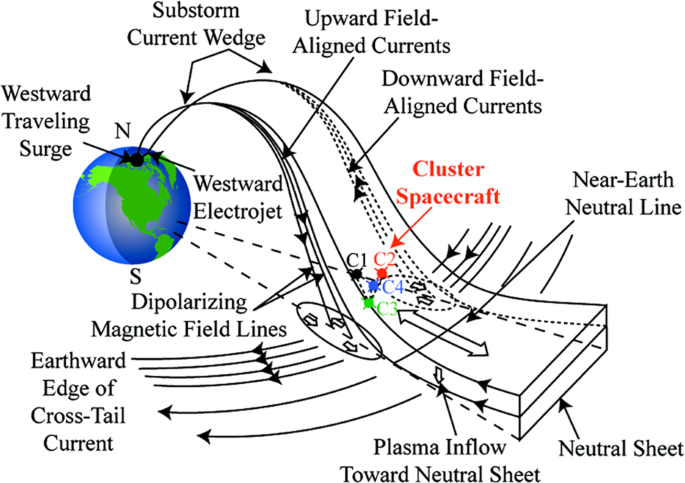
When the magnetic field lines in the tail start to reconnect, part of the plasmasheet will be ejected from the tail and flow Earthward with a speed that often exceeds 400 km/s. The braking of this flow at the inner edge of the plasmasheet requires a substantial \(\mathbf{j}\times\mathbf{B}\) force, and hence a substantial dusk-to-dawn current, which leads to dipolarization of the inner portion of the magnetic field. At the edges of the injection region, this current is diverted into field-aligned currents that drive the auroral electrojet, a strong westward current in the ionosphere. Note that the auroral electrojet via Ohm’s law implies a westward electric field and an equatorward flow of the ionospheric plasma. Flows from the reconnection region and dipolarization of the magnetic field are associated with field-aligned currents coupling to the ionosphere, whose net effect is then the SCW. This sequence of changes, from energy storage through explosive release, is called a magnetospheric substorm. The reconnection process is temporally and spatially varying, which structures the flows in scale sizes of the order of a few \(\mathrm{R}_\mathrm{E}\) and time scales of a few minutes.
Field-aligned auroral currents in the ionosphere are observed to have current densities of \(10\,\mathrm{\mu A}/\mathrm{m}^2\). Considering only field-aligned currents, the current density must decrease higher up where the flux tube widens. At altitudes around \(1\,\mathrm{R}_\mathrm{E}\) the current density is still about \(1\,\mathrm{\mu A}/\mathrm{m}^2\). In the auroral cavity where the electron density \(n_e\) is about \(3\times10^5\,\mathrm{m}^{-3}\), we can estimate the velocity the electrons must have to carry this current as \(v_\parallel=j_\parallel/en_e \sim 2\times10^7\,\mathrm{m/s}\), which corresponds to a kinetic energy slightly higher than 1 keV. When the fast flow injected from the tail by reconnection is stopped, the field-aligned current is carried by electrons that must be accelerated to keV energies. These electrons will cause aurora, and the sudden buildup of this current leads to a breakup of the quiet auroral arc that existed during the growth phase of the substorm.
The auroral breakup occurs in the region of upward field-aligned current, at the western end of the electrojet. The upward current is carried by downgoing electrons that have been accelerated by \(E_\parallel\) at altitudes around \(1\,\mathrm{R}_\mathrm{E}\). When these electrons start to precipitate, a very bright and dynamic auroral display begins. A suitably located observer may see a large part of the sky filled with rapidly moving auroral forms. As illustrated in the classical drawings of an auroral substorm shown by Akasofu 1968 (viewing from the north pole), the aurora spreads poleward, and after a few minutes more stable discrete auroral arcs start to form.
The inertia of the plasma flowing in from the tail with high speed will carry it into a region where the ambient, mainly magnetic, pressure is higher than the pressure in the injected plasma. As the inflow continues the pressure increases, and the injected plasma will start to expand towards the evening and morning side of the magnetosphere. This happens somewhat further from Earth where the ambient magnetic pressure is lower, on field lines that reach the ionosphere poleward of the initial breakup. The azimuthal plasma flows associated with this expansion cause the discrete arcs that form poleward of the breakup.
The simple substorm current wedge model described here is only a crude approximation to the currents that actually exist in space. It is generally believed that the upward current is localized in the premidnight sector while the downward current is more broadly distributed along the auroral oval post-midnight.1 Upward currents are carried by downward moving electrons, while the downward current is a combination of upward flowing electrons and precipitating ions. The actual currents probably do not flow on the same L-shells. It has also been suggested that the current wedge includes currents closing in meridian planes. In this more complex model there is a second current wedge of opposite sense flowing on a lower L-shell with a different current strength. The effect of this loop on the ground is to reduce the apparent strength of the higher latitude current wedge.
The Dungey cycle is the source of the two-cell (DP-2) ionospheric convection pattern. Intervals of steady magnetospheric convection, where the dayside and nightside reconnection rates are roughly balanced, approach the idealized state originally envisioned by Dungey (1961). Yet reconnection is not a steady process, and even during intervals of SMC, when the solar wind driver is relatively constant, plasmasheet convection can be intermittent and bursty. Detailed examination of the responses reveals that a pair of field-aligned currents in the form of a current wedge forms during each of the phenomenological stages. Thus, the SCW system is a key phenomenon across all magnetospheric dynamics related to the Dungey cycle, present from weak to extreme activity conditions, and is the link between magnetospheric dynamics and the ionosphere.
25.4.1 Knight’s relation
By studying the adiabatic motion of electrons in a parallel electric field, Knight [1973] derived a formula for the auroral current-voltage (C-V) relation. Analyzing data from sounding rockets, Lyons et al. [1979] found that the energy flux of precipitating electrons was proportional to the square of the potential drop. Soon after, it was noticed that for the parameters of interest in the upward current region, Knight’s relation could be approximated by [Fridman and Lemaire, 1980] (I feel like this is NOT the original Knight’s relation??? Kosta mentioned the linear relation between FAC and B?) \[ j_{z} \approx -K \Delta\phi \tag{25.1}\] where \(j_z\) is the field-aligned current density below the potential drop and \(\Delta\phi\) is the potential difference between the ionosphere and the equatorial magnetosphere. The constant \(K\), known as the Lyons-Evans-Lundin constant, is given by \[ K=\frac{n_{G}e^2}{\sqrt{2\pi m T_G}} \] where \(N_G\) and \(T_G\) are the density and temperature of electrons in the equatorial generator region. Notice that since \(N_G\) and \(T_G\) may vary in space and time, the term “constant” in this context means “independent of \(\phi\)”. The linear C-V relation Equation 25.1 has since been adopted as a part of theoretical and numerical models. However, there are observations both support and against this relation.
Using a fluid description of the plasma, Rönnmark [1999] showed that within a purely electrostatic quasineutral model the potential drop should be proportional to the square of the upward field-aligned current \[ \Delta \phi = \frac{m_e}{2e^3}\frac{j_z^3}{n^2} \tag{25.2}\] where \(n\) is the density in the acceleration region above the ionosphere.
25.4.2 Current circuit
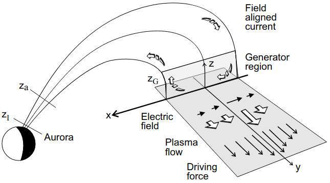
The current circuit connected with a discrete auroral arc is shown in Figure 25.3. Comparing with Figure 25.2 we see that the flows have been rotated from radial to azimuthal. The length scales are also different, since the auroral electrojet is hundreds of kilometers long and the ionospheric current in Figure 25.3 which runs across an auroral arc is at most a few km. Still the physics is very similar. When pointing out some details, we will here use the geometry shown in Figure 25.3.
Let us assume that the auroral flux tube, extending from the ionosphere to the equatorial plane, can be separated into three parts.
- At low altitudes we have the collision dominated ionosphere, where field-aligned currents are connected to horizontal currents.
- The magnetospheric plasma above the ionosphere is collisionless. In a stationary state, and in the absence of collisions, the magnetic moment \(\mu\) and the total energy \(H\) are conserved along the phase-space trajectory of a particle. These assumptions imply that there are no currents perpendicular to the magnetic field lines (???), and the field-aligned current in a flux tube is conserved in the second, main, part of the flux tube.
- The third part is the equatorial generator region. Perpendicular currents are in the generator region driven by kinetic and dynamic pressure gradients, and the divergence of these perpendicular currents is diverted to field-aligned currents. In the real magnetosphere the boundaries between these parts may be rather diffuse, and the generator region may extend far from the equatorial plane.
For simplicity we assume that the main part of an auroral flux tube is separated from the ionosphere and the generator region by well-defined boundaries. Because of quasineutrality, the density of the light and mobile electrons is determined by the ion density. The ion density will remain approximately constant during transitions between different stationary states. Such transitions, for example increases of the field-aligned current, are accomplished by shear Alfvén waves propagating up and down the field lines. The time variation of \(E_\perp\) associated with these Alfvén waves will cause an ion polarization current \(j_\perp\) given by \[ k_\perp = \frac{n_i m_i}{B^2}\frac{\partial E_\perp}{\partial t} \]
Combining this with the ion continuity equation \[ e\frac{\partial n_i}{\partial t} \approx -\partial_\perp j_\perp = \frac{n_i m_i}{B^2}\frac{\partial \partial_\perp E_\perp}{\partial t} \] we can integrate to find the density change \(\Delta n_i\) during the growth of \(E_\perp\). Let \(L_\perp\) be the thickness of the current sheet that \(j_\perp\) connects to. Choosing \(E_\perp=0.1\,\mathrm{V}/\mathrm{m}\) and \(B=10\,\mu\mathrm{T}\) as typical values for the auroral acceleration region we find \[ \bigg\lvert \frac{\Delta n_i}{n_i} \bigg\rvert \sim \frac{m_i}{eB^2}|\partial_\perp E_\perp| \sim \frac{10\,\mathrm{m}}{L_\perp} \]
Clearly, this process can increase the plasma density significantly only within extremely thin current sheets. On the other hand, if the current sheet has a thickness of a few hundred meters or more, the density will remain almost constant. Hence, it seems reasonable to consider the plasma density in the main part of the flux tube as fixed when the current and voltage vary.
In a state of steady field-aligned current the contribution to the current by ions of mass \(m_i\) is about a factor \(\sqrt{m_e/m_i}\) smaller than the contribution by electrons of mass \(m_e\). If we as a first approximation consider this ratio as fixed, the ion and electron currents are separately conserved. In the main part of the flux tube, where the current is purely field-aligned, the plasma density will then be unaffected by the presence of a steady current. However, altitude variations in plasma properties such as ion composition and electron and ion temperatures may cause variations in the ratio between ion and electron current, and this will cause slow decreases or increases of the plasma density.
Pressure forces in the equatorial plane try to establish a strong velocity shear \(\partial_x u_y\), which implies a strong \(\partial_x E_x\) in Figure 25.3 (\(\mathbf{E} = -\mathbf{u}\times\mathbf{B}\)). Recalling eq-ionosphere_potential_derivation we find that the gradient of the ionospheric electric field is determined by the field-aligned current as \[ \frac{\partial E_x}{\partial x} = \frac{j_z}{\Sigma_P} \]
As long as there is no potential drop along the field lines, the magnetospheric and ionospheric electric fields are simply related, and the mapping of a strong velocity shera in the equatorial plane to the ionosphere demands a strong field-aligned current. However, a strong current through the auroral cavity means that the electrons must be accelerated by a potential drop (e.g. Equation 25.2).
The appearance of this potential drop on field lines that carry currents up from the ionosphere means that the ionospheric and magnetospheric electric fields become decoupled. The frozen-in condition does not hold in the acceleration region, and this breakdown of ideal MHD also means that the equatorial plasma is free to flow without dragging the ionosphere along. The potential drop \(\Delta\phi\) limits the current density, and hence the braking \(\mathbf{j}\times\mathbf{B}\) force. Notice that it is the low altitude acceleration in this potential drop, which in the energy spectrum of the precipitating electrons is observed as a peak at the energy \(e\Delta\phi\), that distinguishes the discrete from the diffuse aurora.
The field lines carrying current up from the ionosphere connect to regions with a strong inward gradient of the driving force, which is the outer part of the volume with enhanced pressure. When the brakes in this region are released, the flow will build up a narrower region of high pressure at larger \(y\). ??? Only the outer part of this smaller volume will continue to expand, and this process quickly creates a narrow flow channel in the \(y\)-direction. The outer edge of this channel maps to a discrete auroral arc in the ionosphere.
In the model described above, the flows are constrained to the \(y\)-direction. In the real magnetosphere, the flows can be deviated in the radial \(x\)-direction to form curls and vortices. As illustrated by Akasofu, the geometry of real auroral arcs is very complicated. The patterns are similar to the turbulence seen when water flows from a river into a lake.
I still have many questions regarding the substorms and SCW. Reading the review by (Kepko et al. 2015) makes things worse: my impression is that there has not yet existed a model for explaining the whole current system. No wonder the sawtooth study with MHD-EPIC ended up in a strange way.
25.4.3 Omega Band Auroras
Auroral luminosity undulations of the poleward boundaries of diffuse auroras were first described by Akasofu and Kimball (1964) and were named “omega bands” due to the similarity of their shapes to inverted (poleward-opening) versions of the Greek letter Ω. Omega bands are generally observed in the post-midnight and morning sectors during the recovery phases of magnetospheric substorms. They typically have sizes of 400–1000 km and usually drift eastward at speeds of 0.3–2 km/s.
25.4.4 Theta Auroras
Theta auroras (transpolar aurora arcs) are thought to be linked to high latitude reconnections, which typically happens under northward IMF conditions.
IMF \(B_y\) may also contribute to theta auroras as the twist of magnetic field lines together with high latitude reconnections can lead to the strong aurora arcs.
25.4.5 Throat Auroras
Throat Auroras, named after the finger-like structure on the dayside, are thought to be caused by transient reconnection and magnetopause depression with large \(B_x\) in the cusp region.
25.4.6 Pulsation Auroras
25.5 Region I and Region II Currents
Region II current is linked to the partial ring current around low latitude region. A simple MHD model does not have ring currents (Section 7.9), which means it cannot have Region II currents. Region I currents, however, can be generated, since it relates to the dayside particle precipitation around the polar cap cusp region and reconnection happening at the magnetopause.
Observation indicates that extreme magnetic storms can cause strongly enhanced Region II current compared with Region I current.
25.6 Aurora Oval
- The overall size is very dynamic.
- The size of the oval is more related to the nightside reconnection (as indicated by the nightside contribution of the electric potential). There is no simple relation with the dayside electric potential (CPCP?).
- Fluid model is not enough to explain observation.
25.7 Summary
- Enhanced dayside reconnection
- thin tail current sheet
- reconnection-accelerated electrons
- carry current into the auroral cavity
Up/down direction is determined w.r.t. the ionosphere.↩︎