21 Shock
Shock is a phenomenon that appears when the speed of an object exceeds the characteristic wave speeds. It is characterized by Mach number, the ratio of the shock speed to the characteristic wave speed in the medium. Consider a subsonic disturbance moving through a conventional neutral fluid. As is well-known, sound waves propagating ahead of the disturbance give advance warning of its arrival, and, thereby, allow the response of the fluid to be both smooth and adiabatic. Now, consider a supersonic disturbance. In this case, sound waves are unable to propagate ahead of the disturbance, and so there is no advance warning of its arrival, and, consequently, the fluid response is sharp and non-adiabatic. This type of response is generally known as a shock.
Intuitively, the number of different types of shocks depends on the types of waves in the system. In plasma physics, the simplest system for investigating shocks is ideal MHD. Since information in MHD fluids is carried via three different waves – namely, fast or compressional-Alfvén waves, intermediate or shear-Alfvén waves, and slow or magnetosonic waves – we might expect MHD fluids to support three different types of shocks, corresponding to disturbances traveling faster than each of the aforementioned waves.
In general, a shock propagating through an MHD fluid produces a significant difference in plasma properties on either side of the shock front. The thickness of the front is determined by a balance between convective and dissipative effects. However, dissipative effects in high temperature plasmas are only comparable to convective effects when the spatial gradients in plasma variables become extremely large. Hence, MHD shocks in such plasmas tend to be extremely narrow, and are well-approximated as discontinuities in plasma parameters. The MHD equations, and Maxwell’s equations, can be integrated across a shock to give a set of jump conditions which relate plasma properties on each side of the shock front. If the shock is sufficiently narrow then these relations become independent of its detailed structure. We will derive the jump conditions for a narrow, planar, steady-state, MHD shock in Section 21.1.
The realization of extreme sharpness of a collisionless shock like the Earth’s bow shock immediately posed a serious problem for the MHD description of collisionless shocks. In collisionless MHD there is no known dissipation mechanism that could lead to the observed extremely short transition scales \(\Delta\) in high Mach number flows which are comparable to the ion gyro-radius \(r_\text{Li}\). MHD neglects any differences in the properties of electrons and ions and thus barely covers the very physics of shocks on the observed scales. In the MHD frame, shocks are considered as infinitely narrow discontinuities, narrower than the MHD flow scales \(L\gg \Delta \gg \lambda_d\); on the other hand, these discontinuities must physically be much wider than the dissipation scale \(\lambda_d\) with all the physics going on inside the shock transition. This implies that the conditions derived from collisionless MHD just hold far upstream and far downstream of the shock transition, i.e. far outside the region where the shock interactions are going on. In describing shock waves, collisionless MHD must be used in an asymptotic sense, providing the remote boundary conditions on the shock transition. One must look for processes different from MHD in order to arrive at a description of the processes leading to shock formation and shock dynamics and the structure of the shock transition. In fact, from the MHD single-fluid viewpoint, the shock should not be restricted to the steep shock front, it rather includes the entire shock transition region from outside the foreshock across the shock front down to the boundary layer at the surface of the obstacle. And this holds as well even in two-fluid shock theory that distinguishes between the behaviour of electrons and ions in the plasma fluid. The issue of dissipation is partly indicated in Section 21.1.3.
The basic process of shock formation is the growth of a small disturbance in the plasma by the action of the intrinsic nonlinearity of flow, independent of the cause of the initial disturbance. The latter can be an external driver like a piston or a blast, it can also be an internal instability. Shocks form when nonlinearity causes steepening of the disturbance in space and some processes exists which prevents breaking of the steep wave. Such processes are of dissipative or dispersive nature and are discussed in ascending importance.
It is important to emphasize that the various modes of waves are responsible for the generation of anomalous dissipation, shock ramp broadening, generation of turbulence in the shock environment and shock ramp itself, as well as for particle acceleration, shock particle reflection and the successive effects. The idea is that in a plasma that consists of electrodynamically active particles the excitation of the various plasma wave modes in the EM field as collective effects is the easiest way of energy distribution and transport. There is very little momentum needed in order to accelerate a wave, even though many particles are involved in the excitation and propagation of the wave, much less momentum than accelerating a substantial number of particles to medium energy. Therefore any more profound understanding of shock processes cannot avoid bothering with waves, instabilities, wave excitation and wave-particle interaction.
As a quick summary, in some special cases, for example, shock waves in an ideal neutral gas, the global behavior does not depend on the details of the small-scale physics, because the jump conditions across a hydrodynamic shock are fully determined by the conservation of mass, momentum, and energy. For more complicated systems, such as magnetohydrodynamics with anisotropic ion pressure, the conservation laws constrain the jump conditions, but the pressure anisotropy behind the shock cannot be determined without knowledge of small-scale processes.
A general review of collisionless shocks is given by Balogh and Treumann (2013).
21.1 MHD Theory
The conserved form of MHD equations can be written as: \[ \begin{aligned} \nabla\cdot\mathbf{B}=0 \\ \frac{\partial \mathbf{B}}{\partial t} - \nabla\times (\mathbf{U}\times \mathbf{B})=0 \\ \frac{\partial\rho}{\partial t} + \nabla\cdot(\rho\,\mathbf{U})=0 \\ \frac{\partial (\rho\,\mathbf{U})}{\partial t} + \nabla\cdot\mathbf{S}=0 \\ \frac{\partial K}{\partial t} + \nabla\cdot\mathbf{w}=0 \end{aligned} \tag{21.1}\] where \[ \mathbf{S} = \rho\,\mathbf{U}\,\mathbf{U} + \left(p+ \frac{B^2}{2\mu_0}\right)\mathbf{I}- \frac{\mathbf{B}\mathbf{B}}{\mu_0} \tag{21.2}\] is the total (i.e., including electromagnetic, as well as plasma, contributions) stress tensor1, \(\mathbf{I}\) the identity tensor, \[ K = \frac{1}{2}\rho U^2 + \frac{p}{\gamma-1} + \frac{B^2}{2\mu_0} \tag{21.3}\] the total energy density, and \[ \mathbf{w} = \left(\frac{1}{2}\rho U^2+ \frac{\gamma}{\gamma -1}p\right)\mathbf{U} + \frac{\mathbf{B}\times (\mathbf{U}\times \mathbf{B})}{\mu_0} \tag{21.4}\] the total energy flux density.
Let us move into the rest frame of the shock. For a 1D shock, suppose that the shock front coincides with the \(y\)-\(z\) plane. Furthermore, let the regions of the plasma upstream and downstream of the shock, which are termed regions 1 and 2, respectively, be spatially uniform and time-static, i.e. \(\partial/\partial t = \partial/\partial y = \partial/\partial z = 0\). Moreover, \(\partial/\partial x=0\), except in the immediate vicinity of the shock. Finally, let the velocity and magnetic fields upstream and downstream of the shock all lie in the x-y plane. The situation under discussion is illustrated in the figure below.
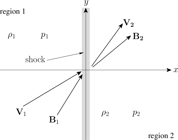
Here, \(\rho_1\), \(p_1\), \(\mathbf{U}_1\), and \(\mathbf{B}_1\) are the downstream mass density, pressure, velocity, and magnetic field, respectively, whereas \(\rho_2\), \(p_2\), \(\mathbf{U}_2\), and \(\mathbf{B}_2\) are the corresponding upstream quantities.2
The basic RH relations are listed in MHD shocks. In the immediate vicinity of the planar shock, Equation 21.1 reduce to \[ \begin{aligned} \frac{\mathrm{d}B_{x}}{\mathrm{d}x}=0 \\ \frac{\mathrm{d}}{\mathrm{d}x}(U_x\,B_y-U_y\,B_x)=0 \\ \frac{\mathrm{d} (\rho\, U_x)}{\mathrm{d}x}=0 \\ \frac{\mathrm{d} S_{xx}}{\mathrm{d}x}=0 \\ \frac{\mathrm{d} S_{xy}}{\mathrm{d}x}=0 \\ \frac{\mathrm{d} w_x}{\mathrm{d}x}=0 \end{aligned} \]
Integration across the shock yields the desired jump conditions: \[ \begin{aligned} \lfloor B_x\rceil=0 \\ \lfloor U_x\,B_y-U_y\,B_x\rceil=0 \\ \lfloor \rho\,U_x\rceil=0 \\ \lfloor \rho\,U_x^{\,2}+p + B_y^{\,2}/2\mu_0\rceil=0 \\ \lfloor \rho\,U_x\,U_y - B_x\,B_y/\mu_0\rceil=0 \\ \Big\lfloor \frac{1}{2}\,\rho\,U^2\,U_x + \frac{\gamma}{\gamma-1}\,p\,U_x + \frac{B_y\,(U_x\,B_y-U_y\,B_x)}{\mu_0}\Big\rceil=0 \end{aligned} \tag{21.5}\] where \(\lfloor A \rceil = A_2 - A_1\) is the difference across the shock. These relations are often called the Rankine-Hugoniot relations for MHD. There are 6 scalar equations and 12 (6 upstream and 6 downstream) scalar variables all together. Assuming that all of the upstream plasma parameters are known, there are 6 unknown parameters in the problem–namely, \(B_{x\,2}\), \(B_{y\,2}\), \(U_{x\,2}\), \(U_{y\,2}\), \(\rho_2\), and \(p_2\). These 6 unknowns are fully determined by the six jump conditions. If we loose the planar assumption, then we typically write the \(x\)-component as the normal component (\(U_n, B_n\)) and the combined y- and z-components as the tangential component (\(U_t,B_t\)): \[ \begin{aligned} \lfloor B_n\rceil=0 \\ \lfloor U_n\,B_t-U_t\,B_n\rceil=0 \\ \lfloor \rho\,U_n\rceil=0 \\ \lfloor \rho\,U_n^{\,2}+p + B_t^{\,2}/2\mu_0\rceil=0 \\ \lfloor \rho\,U_n\,U_t - B_n\,B_t/\mu_0\rceil=0 \\ \Big\lfloor \frac{1}{2}\,\rho\,U^2\,U_n + \frac{\gamma}{\gamma-1}\,p\,U_n + \frac{B_t\,(U_n\,B_t-U_t\,B_n)}{\mu_0}\Big\rceil=0 \end{aligned} \tag{21.6}\]
Luckily this is still deterministic. However, as you can see later, the general case is very complicated.
A clear exposition of the two types of strong discontinuities, namely the shock wave and the tangential discontinuity can be found in §84, Landau & Lifshitz. By definition
- shocks are transition layers across which there is a transport of particles, whereas
- discontinuities are transition layers across which there is no particle transport.
Mathematically, let the shock plane speed be \(U_s\), then \[ \begin{aligned} \lfloor\rho (U_x - U_s)\rceil&\neq 0\quad \text{for shock} \\ \lfloor\rho (U_x - U_s)\rceil&=0\quad \text{for discontinuity} \end{aligned} \tag{21.7}\]
Thus in shocks \(\lfloor U_n \rceil \neq 0\), and in discontinuities \(\lfloor U_n \rceil = 0\). Take a reference frame fixed to the discontinuity with x-axis along the normal. Since mass, momentum and energy is conserved across the discontinuity, we must have from Equation 21.5 for inviscid flows (no magnetic field, y-direction represents the tangential direction), \[ \begin{aligned} \lfloor \rho U_x\rceil=0 \\ \lfloor \rho U_x^2 + p \rceil = 0, \lfloor \rho U_x U_y \rceil=0 \\ \lfloor \rho U_x\left(\frac{1}{2}U^2 + H\right)\rceil=0 \end{aligned} \] where \(H\) is the enthalpy. In tangential discontinuities, no particle transport means \(U_{1x} = U_{2x} = 0\). Then the x-momentum jump implies \(\lfloor p \rceil=0\), where the y-momentum jump sets no restrictions on \(U_y\). There is also no restriction on \(\rho\). Energy equation is also satisfied. Thus, in tangential discontinuities, the density and tangential velocity components can be discontinuities, whereas the pressure must be continuous and the normal velocity component must be zero.
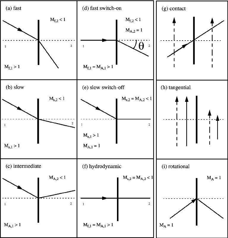
The categories of the solution of Equation 21.5 are shown in Table 21.1. The \(\pm\) signs denote the changes of the downstream compared with the upstream (\(+\) means increase, \(-\) means decrease).
| Type | Particle Transport | \(\rho\) | \(\mathbf{U}\) | \(p\) | \(\mathbf{B}\) | T |
|---|---|---|---|---|---|---|
| Tangential | No | \(\pm\) | \(U_n=0\) | continuous | \(B_n = 0\) | \(\pm\) |
| Contact | No | \(\pm\) | continuous | continuous | continuous | \(\pm\) |
| Slow | Yes | + | - | + | \(B_t\) - | + |
| Intermediate | Yes | continuous | \(\pm\) | \(\pm\) | \(\pm\) | \(\pm\) |
| Rotational | No | continuous | \(U_n=B_n / \sqrt{\mu_0 \rho}\), \(U_t - B_t/\sqrt{\mu_0 \rho}=0\) | continuous | \(B_n = 0\) | \(\pm\) |
| Fast | Yes | + | - | + | \(B_t\) + | + |
The contact discontinuity (CD) is a special case of tangential discontinuity (TD) in which we assume \(\lfloor U_t\rceil = 0\), i.e., the tangential velocity (and so the velocity) is continuous, but not the density and other thermodynamic variables. Since in a CD the thermal pressure remains constant, any change in density must be compensated by a change in temperature. However, a temperature jump is quickly disspated by electron heat conduction, which hints that CD do not persist long. TDs are often observed in the solar wind. The Hot Flow Anomaly (HFA) requires a TD and a normal electric field pointing towards the discontinuity.
The Earth’s magnetopause (Section 22.7.1) is generally a tangential discontinuity. When there is no flux rope been generated, the magnetopause can be treated as the surface of pressure balance between magnetic pressure, ram pressure and thermal pressure. However, when reconnection triggers flux rope generation, it may become a rotational discontinuity (RD) (TO BE CONFIRMED!).
Intermediate (Alfvénic) shocks are incompressive and isentropic. The rotational discontinuity is a special case of the intermediate shock. The tangential velocity relation \(\lfloor \mathbf{U}_t - \frac{\mathbf{B}_t}{\sqrt{\mu_0 \rho}}\rceil=0\) can be derived from Equation 21.6 assuming the Walen relation holds, \(U_n = B_n / \sqrt{\mu_0 \rho}\), i.e. this is an Alfvénic shock. All thermodynamic quantities are continuous across the shock, but the tangential component of the magnetic field can rotate. RD is frequently observed in fast solar wind. Intermediate shocks in general however, unlike rotational discontinuities, can have a discontinuity in the pressure.
Fast- and slow-mode shocks are compressive and are associated with an increase in entropy. Fast/slow shocks have increasing/decreasing magnetic pressure from the upstream to the downstream of the shock. For example, the Earth’s bow shock is a fast, supercritical shock (See criticality in Section 21.1.3).
RD and TD are similar. One easy way to distinguish these two are performing a MVA analysis, get the normal magnetic field component, and see if \(B_N\) (not the jump!) is zero. If \(B_N = 0\), then it is a TD (“tangential” means no normal component); otherwise it is a RD.
The solutions can also be summarized in the context of Riemann problem or visually in Figure 21.2.
21.1.1 Evolutionarity
The hyperbolic nature of the conservation laws allows wave propagation only if it is in accord with causality. Causality is a general requirement in nature, meaning in this case that the drop in speed across a shock must be large enough for the normal component of the downstream flow to fall below the corresponding downstream mode velocity. For a fast shock this implies the following ordering of the normal flow and magnetosonic velocities to both sides of the shock: \[ \begin{aligned} U_\text{1n} > c_\text{1ms}^+ \\ U_\text{2n} < c_\text{2ms}^+ \end{aligned} \] where the numbers 1, 2 refer to upstream and downstream of the fast shock wave.
The first condition is necessary for the shock to be formed as a priori; it is the second condition which (partially) accounts for the evolutionarity. Otherwise the small fast-mode disturbances excited downstream and moving upward towards the shock would move faster than the flow, they would overcome the shock and steepen it without limit. Since this cannot happen for a shock to form, the downstream normal speed must be less than the downstream fast magnetosonic speed. Furthermore, for fast shocks the flow velocity must be greater than the intermediate (Alfvén) speed on both sides of the shock, while for slow shocks it must be less than the intermediate speed on both sides. These conditions hold because of the same reason as otherwise the corresponding waves would catch up with the shock front, modify and destroy it and no shock could form.
21.1.2 Coplanarity
For a stationary ideal MHD shock wave with no other wave activity or kinetic processes present outside the shock transition, such that dissipation takes place solely inside the narrow shock transition and this transition region can be considered as infinitesimally thin with respect to all other physical scales in the plasma, the electric field in the shock rest frame is strictly perpendicular to the magnetic field, \(\mathbf{E} = -\mathbf{U}\times\mathbf{B}\). The stationary Faraday’s law \[ \nabla\times\mathbf{E} = \dot{\mathbf{B}} = 0 \] leads to the vanishing of the difference in the tangential components of the magnetic field to both sides \[ (U_{n2} - U_{n1})(\mathbf{B}_{t2}\times\mathbf{B}_{t1}) = 0 \]
For a shock \(\lfloor U_n \rceil \neq 0\), hence \[ \mathbf{B}_{t2}\times\mathbf{B}_{t1} = 0 \] i.e. the two tangential components to both sides are strictly parallel.
With more details, \(\lfloor U_t \rceil\) from the RH relations and obtain \[ \lfloor U_n \mathbf{B}_t \rceil = \frac{B_n^2}{\mu_0 ... }\lfloor \mathbf{B}_t \rceil \]
Hence the cross product of the left with the right hand side must vanish: \[ \begin{aligned} \lfloor \mathbf{B}_t \rceil \times \lfloor U_n\mathbf{B}_t \rceil = 0 \\ (\mathbf{B}_{t2} - \mathbf{B}_{t1})\times(U_{n2}\mathbf{B}_{t2} - U_{n1}\mathbf{B}_{t1}) = 0 \\ (U_{n1} - U_{n2})(\mathbf{B}_{t1}\times\mathbf{B}_{t2}) = 0 \\ \mathbf{B}_{t1} \parallel \mathbf{B}_{t2} \end{aligned} \tag{21.8}\]
The resulting coplanarity theorem implies that the magnetic field across the shock has a reduced 2-D geometry: upstream and dowstream tangential fields are parallel to each other and coplanar with the shock normal \(\hat{n}\).
Coplanarity does not strictly hold, however. For instance, when the shock is non-stationary, i.e. when its width changes with time or in the direction tangential to the shock, then in Faraday’s law \(\partial\mathbf{B}/\partial t = \nabla\times\mathbf{E} \neq 0\), and coplanarity becomes violated.
Also, any upstream low frequency EM wave that propagates along the upstream magnetic field, possesses a magnetic wave field that is perpendicular to the upstream field. When it encounters the shock, this tangential component will be transformed and amplified across the shock. This naturally introduces an out-of-plane magnetic field component, thereby violating the co-planarity condition. There are also other effects which violate coplanarity at a non-MHD shock.
21.1.3 Criticality
Shock is a dissipative structure in which the kinetic and magnetic energy of a directed plasma flow is partly transferred to heating of the plasma. The dissipation does not take place, however, by means of particle collisions for a shock in space. Collisionless shocks can be divided into super- and sub-critical, according to their Mach-numbers \(M < M_c\) being smaller or \(M > M_c\) larger than some critical Mach-number \(M_c\). \(M_c\) refers to a threshold value of the shock’s Mach number above which certain physical processes become dominant, leading to distinct changes in the shock’s behavior and structure.3
Depending on the specific physical processes, we can have different critical Mach numbers associated with collisionless shocks:
\(M_c\) for electron injection: This is the minimum Mach number above which thermal electrons in the upstream plasma can be accelerated to high energies and injected into the shock acceleration process. This injection is essential for producing the observed cosmic ray electron spectra.
\(M_c\) for ion reflection: This is the minimum Mach number above which a significant fraction of upstream ions are reflected from the shock front. This ion reflection plays a crucial role in the shock dissipation process and can lead to the formation of foreshocks.
\(M_c\) for whistler precursor formation: This is the minimum Mach number above which whistler waves can be excited upstream of the shock, forming a precursor wave structure that can modify the shock’s properties.
\(M_c\) for nonlinear wave steepening: This is the minimum Mach number above which non-linear wave steepening effects become important, leading to the formation of solitons and other non-linear wave structures in the shock transition region.
For a resistive MHD shock Marshall [1955] had numerically determined the critical Mach number to \(M_c\approx 2.76\) (see Figure 21.3). In various scenarios, \(M_c\) typically fall in the range of 2-10 for most astrophysical and space plasma environments.
Subcritical shocks are capable of generating sufficient dissipation to account for retardation, thermalisation and entropy in the time the flow crosses the shock from upstream to downstream. The relevant processes are based on wave-particle interaction between the shocked plasma and the shock-excited turbulent wave fields.
For supercritical shocks this is, however, not the case. Supercritical shocks must evoke mechanisms different from simple wave-particle interaction for getting rid of the excess energy in the bulk flow that cannot be dissipated by any classical anomalous dissipation. Above the critical Mach number the simplest efficient way of energy dissipation is rejection of the inflowing excess energy from the shock by reflecting a substantial part of the incoming plasma back upstream. The non-thermal processes for dissipating excess energy include
- Particle acceleration to very high energies;
- Generation of strong, complex magnetic fields;
- Significant heating of the plasma.
To show how the critical Mach number of a shock arises from the Rankine-Hugoniot relations we consider the strictly perpendicular case with vanishing upstream pressure \(P_1 = 0\). The jump conditions become very simple in this case: \[ \begin{aligned} n_1 U_1 &= n_2 U_2 \\ v_1 B_1 &= v_2 B_2 \\ n_1 U_1^2 + \frac{B_1^2}{2\mu_0 m} &= n_2 U_2^2 + \frac{P_2}{m} + \frac{B_2^2}{2\mu_0 m} \\ \frac{U_1^2}{2} + \frac{B_1^2}{\mu_0 m n_1} &= \frac{U_2^2}{2} + \frac{\gamma}{\gamma - 1}\frac{P_2}{m n_2} + \frac{B_1^2}{\mu_0 m n_1} \end{aligned} \] where \(B\) is the only existing tangential component of the magnetic field here, and \(\gamma = 5/3\) is the adiabatic index (valid for fast, adiabatic transitions across the shock). This is the simplest imaginable case of an MHD shock, and it is easy to solve these equations. Figure 21.3 shows the resulting relation between the normalised downstream flow \(U_2/U_1\) and downstream sound speed \(c_{s2}/U_1 = \sqrt{\gamma P_2/n_2}/ v_1\) as function of upstream Alfvén Mach number \(M_A = U_1 \sqrt{\mu_0 m n_1} / B_1\).
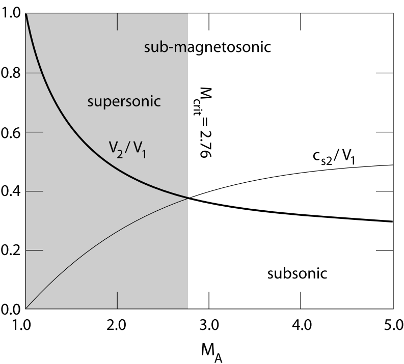
The two curves in the figure cross each other at the critical Mach number which in the present case is \(M_c = 2.76\) and where the downstream sound speed exceeds the flow speed. Below the critical Mach number the downstream flow is still supersonic (though clearly sub-magnetosonic!). Only above the critical Mach number the downstream flow velocity falls below the downstream sound speed. There is thus a qualitative change in the shock character above it that is not contained in the Rankine-Hugoniot conditions.
So as a quick recap, the inflow of matter into a supercritical shock is so fast that the time scales on which dissipation would take place are too long for dissipating the excess energy and lowering the inflow velocity below the downstream magnetosonic velocity. Hence, the condition for criticality, is that the downstream flow velocity becomes equal to the downstream sonic speed, which yielded the critical Mach number, \(M_c \simeq 2.76\).
The determination of the critical Mach number poses an interesting question of why sonic speed appears in the downstream. The finite magnetic field compression ratio sets an upper limit to the rate of resistive dissipation that is possible in an MHD shock. Plasmas possess several dissipative lengths, depending on which dissipative process is considered. Any nonlinear wave that propagates in the plasma should steepen as long, until its transverse scale approaches the longest of these dissipative scales. Then dissipation sets on and limits its amplitude.
Thus, when the wavelength of the fast magnetosonic wave approaches the resistive length, the magnetic field decouples from the wave by resistive dissipation, and the wave speed becomes the sound speed downstream of the shock ramp. The condition for the critical Mach number is then given by \(U_{n2} = c_{2s}\). Similarly, for the slow-mode shock, because of its different dispersive properties, the resistive critical-Mach number is defined by the condition \(U_{1n} = c_{1s}\)4. Since these quantities depend on wave angle, they have to be solved numerically. Prior studies showed that critical fast-mode Mach number varies between 1 and 3, depending on the upstream plasma parameters and flow angle to the magnetic field. It is usually called first critical Mach number, because there is theoretical evidence in simulations for a second critical Mach number, which comes into play when the shock structure becomes time dependent, whistlers accumulate at the shock front and periodically cause its reformation. The dominant dispersion is then the whistler dispersion. An approximate expression for this second or whistler critical Mach number is \[ M_{2c} \propto \left( \frac{m_i}{m_e} \right)^{1/2}\cos\theta_{Bn} \tag{21.9}\] where the constant of proportionality depends on whether one defines the Mach number with respect to the whistler phase or group velocities. For the former it is \(1/2\), and for the latter \(\sqrt{27/64}\) [Oka+, 2006].
It is clear that it is the smallest critical Mach number that determines the behaviour of the shock. In simple words: \(M > 1\) is responsible for the existence of the shock under the condition that an obstacle exists in the flow, which is disturbed in some way such that fast waves can grow, steepen and form shocks. When, in addition, the flow exceeds the next lowest Mach number for a given \(\theta_{Bn}\) the shock at this angle will make the transition into a supercritical shock and under additional conditions, which have not yet be ultimately clarified, will start reflecting particles back upstream. If, because of some reason, this would not happen, the flow might have to exceed the next higher critical Mach number until reflection becomes possible. In such a case the shock would become metastable in the region where the Mach number becomes supercritical, will steepen and shrink in width until other effects and – ultimately – reflection of particles can set on.
21.1.4 Parallel Shock
The first special case is the so-called parallel shock in which both the upstream and downstream plasma flows are parallel to the magnetic field, as well as perpendicular to the shock front. In other words, \[ \begin{aligned} \mathbf{U}_1 = (U_1,\,0,\,0),\quad\mathbf{U}_2 = (U_2,\,0,\,0) \\ \mathbf{B}_1 = (B_1,\,0,\,0),\quad\mathbf{B}_2 = (B_2,\,0,\,0) \end{aligned} \tag{21.10}\]
Substitution into Equation 21.5 yields \[ \begin{aligned} \frac{B_2}{B_1} &= 1\\ \frac{\rho_2}{\rho_1} &= r \\ \frac{U_2}{U_1} &= r^{-1} \\ \frac{p_2}{p_1} &= R \\ \end{aligned} \tag{21.11}\] with \[ \begin{aligned} r &= \frac{(\gamma + 1)M_1^2}{2+(\gamma-1)M_1^2} \\ R &= 1 + \gamma M_1^2 (1-r^{-1}) = \frac{(\gamma+1)r - (\gamma-1)}{(\gamma+1) - (\gamma-1)r} \end{aligned} \tag{21.12}\]
Here, \(M_1 = U_1/c_{s1}\), where \(c_{s1} = \sqrt(\gamma p_1/\rho_1)\) is the upstream sound speed. Thus, the upstream flow is supersonic if \(M_1>1\), and subsonic if \(M_1<1\). Incidentally, as is clear from the above expressions, a parallel shock is unaffected by the presence of a magnetic field. In fact, this type of shock is identical to that which occurs in neutral fluids, and is, therefore, usually called a hydrodynamic shock.
It is easily seen from Equation 21.10 that there is no shock (i.e., no jump in plasma parameters across the shock front) when the upstream flow is exactly sonic: i.e., when \(M_1=1\). In other words, \(r=R=1\) when \(M_1=1\). However, if \(M_1\neq 1\) then the upstream and downstream plasma parameters become different (i.e., \(r\neq 1\), \(R\neq 1\)) and a true shock develops. In fact, it is easily demonstrated that \[ \begin{aligned} \frac{\gamma-1}{\gamma+1} &\leq r \leq \frac{\gamma+1}{\gamma-1} \\ 0&\leq R \leq \infty \\ \frac{\gamma-1}{2\,\gamma}&\leq M_1^2\leq \infty \end{aligned} \tag{21.13}\]
Note that the upper and lower limits in the above inequalities are all attained simultaneously.
The previous discussion seems to imply that a parallel shock can be either compressive (i.e., \(r>1\)) or expansive (i.e., \(r<1\)). Is there a preferential direction across the shock? In other words, can we tell the upstream and the downstream? Yes, with the additional physics principle of the second law of thermodynamics. This law states that the entropy of a closed system can spontaneously increase, but can never spontaneously decrease. Now, in general, the entropy per particle is different on either side of a hydrodynamic shock front. Accordingly, the second law of thermodynamics mandates that the downstream entropy must exceed the upstream entropy, so as to ensure that the shock generates a net increase, rather than a net decrease, in the overall entropy of the system, as the plasma flows through it.
The (suitably normalized) entropy per particle of an ideal plasma takes the form \[ S = \ln\left(\frac{p}{\rho^\gamma}\right) \]
Hence, the difference between the upstream and downstream entropies is \[ \lfloor S\rceil =\ln R - \gamma\,\ln r \]
Now, using Equation 21.12, \[ r\frac{\mathrm{d}\lfloor S \rceil}{dr} = \frac{r}{R}\frac{dR}{dr} - \gamma = \frac{\gamma(\gamma^2-1)(r-1)^2}{[(\gamma+1)r - (\gamma-1)][(\gamma+1)-(\gamma-1)r]} \]
Furthermore, it is easily seen from Equation 21.13 that \(\mathrm{d}\lfloor S \rceil/dr\ge 0\) in all situations of physical interest. However, \(\lfloor S \rceil = 0\) when \(r=1\), since, in this case, there is no discontinuity in plasma parameters across the shock front. We conclude that \(\lfloor S \rceil<0\) for \(r<1\), and \(\lfloor S \rceil>0\) for \(r>1\). It follows that the second law of thermodynamics requires hydrodynamic shocks to be compressive: i.e., \(r\equiv\rho_2 / \rho_1>1\). In other words, the plasma density must always increase when a shock front is crossed in the direction of the relative plasma flow. It turns out that this is a general rule which applies to all three types of MHD shock. In the shock rest frame, the shock is associated with an irreversible (since the entropy suddenly increases) transition from supersonic to subsonic flow.
The upstream Mach number, \(M_1\), is a good measure of shock strength: i.e., if \(M_1=1\) then there is no shock, if \(M_1-1 \ll 1\) then the shock is weak, and if \(M_1\gg 1\) then the shock is strong. We can define an analogous downstream Mach number, \(M_2=U_2/(\gamma\,p_2/\rho_2)^{1/2}\). It is easily demonstrated from the jump conditions that if \(M_1>1\) then \(M_2 < 1\). In other words, in the shock rest frame, the shock is associated with an irreversible (since the entropy suddenly increases) transition from supersonic to subsonic flow. Note that \(r\equiv \rho_2/\rho_1\rightarrow (\gamma+1)/(\gamma-1)\), whereas \(R\equiv p_2/p_1\rightarrow\infty\), in the limit \(M_1\rightarrow \infty\). In other words, as the shock strength increases, the compression ratio, \(r\), asymptotes to a finite value, whereas the pressure ratio, \(P\), increases without limit. For a conventional plasma with \(\gamma=5/3\), the limiting value of the compression ratio is 4: i.e., the downstream density can never be more than four times the upstream density. We conclude that, in the strong shock limit, \(M_1\gg 1\), the large jump in the plasma pressure across the shock front must be predominately a consequence of a large jump in the plasma temperature, rather than the plasma density. In fact, the definitions of \(r\) and \(R\) imply that \[ \frac{T_2}{T_1}\equiv \frac{R}{r}\rightarrow \frac{2\gamma(\gamma-1)M_1^2}{(\gamma+1)^2}\gg 1 \] as \(M_1\rightarrow\infty\). Thus, a strong parallel, or hydrodynamic, shock is associated with intense plasma heating.
As we have seen, the condition for the existence of a hydrodynamic shock is \(M_1>1\), or \(U_1 > U_{S\,1}\). In other words, in the shock frame, the upstream plasma velocity, \(U_1\), must be supersonic. However, by Galilean invariance, \(U_1\) can also be interpreted as the propagation velocity of the shock through an initially stationary plasma. It follows that, in a stationary plasma, a parallel, or hydrodynamic, shock propagates along the magnetic field with a supersonic velocity.
21.1.5 Perpendicular Shock
The second special case is the so-called perpendicular shock in which both the upstream and downstream plasma flows are perpendicular to the magnetic field, as well as the shock front. In other words, \[ \begin{aligned} \mathbf{U}_1 = (U_1,\,0,\,0),\quad\mathbf{U}_2 = (V_2,\,0,\,0) \\ \mathbf{B}_1 = (0,\,B_1,\,0),\quad\mathbf{B}_2 = (0,\,B_2,\,0) \end{aligned} \tag{21.14}\]
Substitution into Equation 21.5 yields \[ \begin{aligned} \frac{B_2}{B_1} &= r\\ \frac{\rho_2}{\rho_1} &= r \\ \frac{U_2}{U_1} &= r^{-1} \\ \frac{p_2}{p_1} &= R \\ \end{aligned} \tag{21.15}\] where \[ R = 1+ \gamma\,M_1^{\,2}\,(1-r^{-1}) + \beta_1^{-1}\,(1-r^2) \tag{21.16}\] and \(r\) is a real positive root of the quadratic \[ F(r) = 2\,(2-\gamma)\,r^2+ \gamma\,[2\,(1+\beta_1)+ (\gamma-1)\beta_1 M_1^2]r - \gamma\,(\gamma+1)\,\beta_1\,M_1^2=0 \tag{21.17}\]
Here, \(\beta_1 = 2\mu_0 p_1/B_1^2\).
Now, if \(r_1\) and \(r_2\) are the two roots of Equation 21.17 then \[ r_1 r_2 = -\frac{\gamma(\gamma+1)\beta_1 M_1^2}{2(2-\gamma)} \]
Assuming that \(\gamma < 2\), we conclude that one of the roots is negative, and, hence, that Equation 21.17 only possesses one physical solution: i.e., there is only one type of MHD shock which is consistent with Equation 21.14. Now, it is easily demonstrated that \(F(0)<0\) and \(F(\gamma+1/\gamma-1)>0\). Hence, the physical root lies between \(r=0\) and \(r=(\gamma+1)/(\gamma-1)\).
Using similar analysis to that employed in the previous subsection, it is easily demonstrated that the second law of thermodynamics requires a perpendicular shock to be compressive: i.e., \(r>1\). It follows that a physical solution is only obtained when \(F(1)<0\), which reduces to \[ M_1^{\,2} > 1 + \frac{2}{\gamma\,\beta_1} \]
This condition can also be written \[ \mathbf{U}_1^2 > \mathbf{V}_{s1}^2 + \mathbf{V}_{A1}^2 = V_{+\,1}^2 \] where \(V_{A1} = B_1/\sqrt(\mu_0 \rho_1)\) is the upstream Alfvén speed. \(V_{+\,1} = (V_{S\,1}^{\,2} + V_{A\,1}^{\,2})^{1/2}\) can be recognized as the velocity of a fast wave propagating perpendicular to the magnetic field (Section 10.7.4). Thus, the condition for the existence of a perpendicular shock is that the relative upstream plasma velocity must be greater than the upstream fast wave velocity. Incidentally, it is easily demonstrated that if this is the case then the downstream plasma velocity is less than the downstream fast wave velocity. We can also deduce that, in a stationary plasma, a perpendicular shock propagates across the magnetic field with a velocity which exceeds the fast wave velocity.
In the strong shock limit, \(M_1\gg 1\), Equation 21.16 and Equation 21.17 become identical to Equation 21.12. Hence, a strong perpendicular shock is very similar to a strong hydrodynamic shock (except that the former shock propagates perpendicular, whereas the latter shock propagates parallel, to the magnetic field). In particular, just like a hydrodynamic shock, a perpendicular shock cannot compress the density by more than a factor \((\gamma+1)/(\gamma-1)\). However, according to Equation 21.15, a perpendicular shock compresses the magnetic field by the same factor that it compresses the plasma density. It follows that there is also an upper limit to the factor by which a perpendicular shock can compress the magnetic field.
21.1.6 Oblique Shock
Let us now consider the general case in which the plasma velocities and the magnetic fields on each side of the shock are neither parallel nor perpendicular to the shock front. It is convenient to transform into the so-called de Hoffmann-Teller frame in which \(|\mathbf{U}_1\times \mathbf{B}_1|=0\), or \[ U_{x1}B_{y1} - U_{y1}B_{x1} = 0 \tag{21.18}\]
In other words, it is convenient to transform to a frame which moves at the local \(\mathbf{E}\times\mathbf{B}\) velocity of the plasma. The key idea is to extract the velocity component perpendicular to \(\mathbf{B}_1\) from \(\mathbf{v}_1\). One temptive idea is to just remove the perpendicular part: \[ \begin{aligned} \mathbf{V}_{\mathrm{dHT}} = \mathbf{U}_1 - (\mathbf{U}_1 \cdot \mathbf{b}_1)\mathbf{b}_1 \\ \mathbf{U}_1^\prime = \mathbf{U}_1 - \mathbf{V}_\mathrm{dHT} = (\mathbf{U}_1 \cdot \mathbf{b}_1)\mathbf{b}_1 \end{aligned} \]
Note that the transformation is not unique, since one can always add a parallel velocity component. Although the above transformation is correct, it introduces two issues:
- The ram pressure \(\rho V_n^2\) is changed between the two coordinates.
- Equation 21.22 may not possess a valid solution given certain parameters (e.g. \(\mathrm{MA}_1 = 5, \theta_1 = 65^\circ\) will give \(r<1\).)
To fix this, we can use another transformation: \[ \begin{aligned} \mathbf{V}_{\mathrm{dHT}} = \mathbf{U}_1 - \frac{U_x}{B_x}\mathbf{B} \\ \mathbf{U}_1^\prime = \mathbf{U}_1 - \mathbf{V}_\mathrm{dHT} = \frac{U_x}{B_x}\mathbf{B} \end{aligned} \tag{21.19}\]
A nice property of this transformation is that the normal velocity component is kept the same, so is the ram pressure. Therefore, we can apply the same quantities in the lab frame as in the de Hoffmann-Teller frame.
Taking Equation 21.18 into the 2nd jump condition of Equation 21.5 gives \[ U_{x2}B_{y2} - U_{y2}B_{x2} = 0 \tag{21.20}\] or \(|\mathbf{U}_2\times \mathbf{B}_2|=0\). Thus, in the de Hoffmann-Teller frame, the upstream plasma flow is parallel to the upstream magnetic field, and the downstream plasma flow is also parallel to the downstream magnetic field. Furthermore, the magnetic contribution to the jump condition Equation 21.5 (last eq.) becomes identically zero, which is a considerable simplification.
Equation 21.18 and Equation 21.20 can be combined with the general jump conditions Equation 21.5 to give5 \[ \begin{aligned} \frac{\rho_2}{\rho_1}&=r \\ \frac{B_{x\,2}}{B_{x\,1}} &= 1 \\ \frac{B_{y\,2}}{B_{y\,1}} &= r\frac{U_{1}^{2} - V_{A\,1}^{2}}{U_{1}^{2} - r\,V_{A\,1}^{2}} \\ \frac{U_{x\,2}}{U_{x\,1}} &= \frac{1}{r} \\ \frac{U_{y\,2}}{U_{y\,1}} &= \frac{U_{1}^{2} - V_{A\,1}^{2}}{U_{1}^{2}-r\,V_{A\,1}^{2}} \\ \frac{p_2}{p_1} &= 1+\frac{\gamma U_1^2 (r-1)}{V_{s1}^2 r}\left[\cos^2\theta_1 - \frac{r V_{A1}^2 \sin^2\theta_1[(r+1)U_1^2 - 2r V_{A1}^2]}{2(U_1^2 - r\,V_{A\,1}^2)^2} \right] \end{aligned} \tag{21.21}\] where \(U_{x,1}=U_1\cos\theta_1\) is the component of the upstream velocity normal to the shock front, and \(\theta_1\) is the angle subtended between the upstream plasma flow and the shock front normal.67 Finally, given the compression ratio, \(r\), the square of the normal upstream velocity, \(U_1^{\,2}\), is a real root of a cubic equation known as the shock adiabatic:8 \[ \begin{aligned} 0 = & (U_{1}^2 - r V_{A1}^2)^2\{ [(\gamma+1) - (\gamma-1)r]U_{1}^2\cos^2\theta_1 - 2r V_{s1}^2 \} \\ & -r\sin^2\theta_1 U_{1}^2 V_{A1}^2 \{ [\gamma+(2-\gamma)r]U_{1}^2 - [(\gamma+1) - (\gamma-1)r]r\, V_{A1}^2 \} \end{aligned} \tag{21.22}\]
As before, the second law of thermodynamics mandates that \(r>1\).
Weak shock limit
Let us first consider the weak shock limit \(r\rightarrow 1\). In this case, it is easily seen that the three roots of the shock adiabatic reduce to the slow, intermediate (or Shear-Alfvén), and fast waves, respectively, propagating in the normal direction to the shock front: \[ \begin{aligned} U_1^{\,2}&=V_{-\,1}^{\,2}\equiv \frac{V_{A\,1}^{\,2}+V_{S\,1}^{\,2}- [(V_{A\,1}+V_{S\,1})^2 -4\,\cos^2\theta_1\,V_{S\,1}^{\,2}\,V_{A\,1}^{\,2}]^{1/2}}{2} \\ U_1^{\,2}&=\cos^2\theta_1\,V_{A\,1}^{\,2} \\ U_1^{\,2}&=V_{+\,1}^{\,2}\equiv \frac{V_{A\,1}^{\,2}+V_{S\,1}^{\,2} + [(V_{A\,1}+V_{S\,1})^2 -4\,\cos^2\theta_1\,V_{S\,1}^{\,2}\,V_{A\,1}^{\,2}]^{1/2}}{2} \end{aligned} \]
We conclude that slow, intermediate, and fast MHD shocks degenerate into the associated MHD waves in the limit of small shock amplitude. Conversely, we can think of the various MHD shocks as nonlinear versions of the associated MHD waves. It is easily demonstrated that \[ V_{+1} > \cos\theta_1 V_{A1} > V_{-1} \]
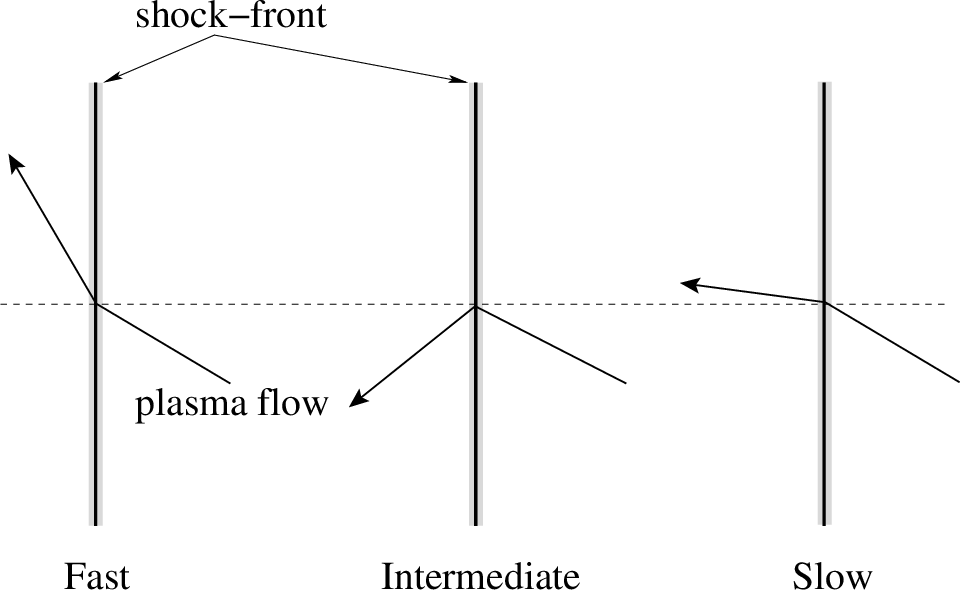
In other words, a fast wave travels faster than an intermediate wave, which travels faster than a slow wave. It is reasonable to suppose that the same is true of the associated MHD shocks, at least at relatively low shock strength. It follows from Equation 21.21 that \(B_{y2}>B_{y1}\) for a fast shock, whereas \(B_{y\,2}<B_{y\,1}\) for a slow shock. For the case of an intermediate shock, we can show, after a little algebra, that \(B_{y\,2}\rightarrow -B_{y\,1}\) in the limit \(r\rightarrow 1\). We can conclude that (in the de Hoffmann-Teller frame) fast shocks refract the magnetic field and plasma flow (recall that they are parallel in our adopted frame of the reference) away from the normal to the shock front, whereas slow shocks refract these quantities toward the normal. Moreover, the tangential magnetic field and plasma flow generally reverse across an intermediate shock front. This is illustrated in Figure 21.4.
When \(r\) is slightly larger than unity it is easily demonstrated that the conditions for the existence of a slow, intermediate, and fast shock are \(U_1> V_{-\,1}\), \(U_1> \cos\theta_1\,V_{A\,1}\), and \(U_1> V_{+\,1}\), respectively.
Strong shock limit
Let us now consider the strong shock limit, \(U_1^{\,2}\gg 1\). In this case, the shock adiabatic yields \(r\rightarrow r_m=(\gamma+1)/(\gamma-1)\), and \[ U_1^{\,2} \simeq \frac{r_m}{\gamma-1}\,\frac{2V_{S1}\sin^2\theta_1\,[\gamma + (2-\gamma)\,r_m]\,V_{A1}^2}{r_m-r} \]
There are no other real roots. The above root is clearly a type of fast shock. The fact that there is only one real root suggests that there exists a critical shock strength above which the slow and intermediate shock solutions cease to exist. (In fact, they merge and annihilate one another.) In other words, there is a limit to the strength of a slow or an intermediate shock. On the other hand, there is no limit to the strength of a fast shock. Note, however, that the plasma density and tangential magnetic field cannot be compressed by more than a factor \((\gamma+1)/(\gamma-1)\) by any type of MHD shock.
\(\theta_1=0\)
Consider the special case \(\theta_1=0\) in which both the plasma flow and the magnetic field are normal to the shock front. In this case, the three roots of the shock adiabatic are \[ \begin{aligned} U_1^2&=\frac{2r\,V_{S1}^2}{(\gamma+1)-(\gamma-1)\,r} \\ U_1^2&=r\,V_{A1}^2 \\ U_1^2&=r\,V_{A1}^2 \end{aligned} \]
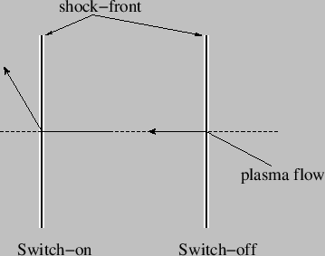
We recognize the first of these roots as the hydrodynamic shock discussed in Section 21.1.4. This shock is classified as a slow shock when \(V_{S\,1}<V_{A\,1}\), and as a fast shock when \(V_{S\,1}> V_{A\,1}\). The other two roots are identical, and correspond to shocks which propagate at the velocity \(U_1 =\sqrt{r}\, V_{A\,1}\) and “switch-on” the tangential components of the plasma flow and the magnetic field: it can be seen from Equation 21.21 that \(U_{y\,1}=B_{y\,1} =0\) whilst \(U_{y\,2}\neq 0\) and \(B_{y\,2}\neq 0\) for these types of shock.
There we have “switch-on” and “switch-off” shocks which refer to the generation and elimination of tangential components of the plasma flow and the magnetic field. Incidentally, it is also possible to have a “switch-off” shock which eliminates the tangential components of the plasma flow and the magnetic field. According to Equation 21.21, such a shock propagates at the velocity \(U_1=\cos\theta_1\,V_{A\,1}\)9. Switch-on and switch-off shocks are illustrated in Figure 21.5.
\(\theta_1=\pi/2\)
Consider another special case \(\theta_1=\pi/2\). As is easily demonstrated, the three roots of the shock adiabatic are \[ \begin{aligned} U_1^{\,2}&=r \left(\frac{2V_{S1}^2 + [\gamma+(2-\gamma)\,r]\,V_{A1}^2} {(\gamma+1)-(\gamma-1)\,r}\right)\\ U_1^{\,2}&=0 \\ U_1^{\,2}&=0 \end{aligned} \]
The first of these roots is clearly a fast shock, and is identical to the perpendicular shock discussed in Section 21.1.5, except that there is no plasma flow across the shock front in this case. (IS IT BECAUSE OF THE HT FRAME?) The fact that the two other roots are zero indicates that, like the corresponding MHD waves, slow and intermediate MHD shocks do not propagate perpendicular to the magnetic field.
MHD shocks have been observed in a large variety of situations. For instance, shocks are known to be formed by supernova explosions, by strong stellar winds, by solar flares, and by the solar wind upstream of planetary magnetospheres.
21.1.7 Switch-On and Switch-Off Shocks
Parallel shocks in MHD should, theoretically, behave exactly like gasdynamic shocks, not having any upstream tangential magnetic field component and should also not have any downstream tangential field. This conclusion does not hold rigourously, however, since plasmas consist of charged particles which are sensitive to fluctuations in the field and can excite various waves in the plasma via electric currents which then become the sources of magnetic fields. The kinetic effects in parallel and quasi-parallel shocks play an important role in their physics and are well capable of generating tangential fields at least on scales shorter than the ion scale.
However, even in MHD as we have seen in the previous subsection, one stumbles across the interesting fact that this kind of shocks must have peculiar properties. The reason is that they are not, as in gasdynamics, the result of steepened sound waves, in which case they would simply be purely electrostatic shocks. At the contrary, the waves propagating parallel to the magnetic field are Alfvén and magnetosonic waves. Alfvén waves contain transverse magnetic field components. These transverse wave fields, in a parallel shock, are in fact tangential to the shock. Hence, if a purely parallel shock steepens, the transverse Alfvén waves do steepen as well, and the shock after the transition from upstream to downstream switches on a tangential magnetic component which originally was not present. Such shocks are called switch-on shocks. Similarly one can imagine the case that a tangential component behind the shock is by the same process switched off by an oppositely directed switch-on field, yielding a switch-off shock.
The problem of whether or not such shocks exist in MHD is related to the question whether or not an Alfvén wave steepens nonlinearly when propagating into a shock. To first order this steepening for an ordinary Alfvén wave is zero. However, to second order a wave trailing the leading Alfvén wave feels its weak transverse magnetic component. This trailing wave therefore propagates slightly oblique to the main magnetic field and thus causes a second order density compression which in addition to generating a shock-like plasma compression changes the Alfvén velocity locally. In the case when the trailing wave is polarised in the same direction as the leading wave it also increases the transverse magnetic field component downstream of the compression thereby to second order switching on a tangential magnetic component. A whole train of trailing waves of same polarisation will thus cause strong steepening in both the density and tangential magnetic field.
Clearly, this kind of shocks is a more or less exotic case of MHD shocks whose importance is not precisely known, with very rare cases of observation.
21.2 Double Adiabatic MHD
The classical approach by Chew et al. (1956) utilizes the MHD framework by assuming isotropic distributions parallel and perpendicular to the magnetic field, which results in scalar pressures on the two sides of the shock. This is now known as the CGL or double adiabatic theory.
When we shift to the MHD with anisotropic pressure tensor \[ P_{ij} = p_\perp \delta_{ij} + (p_\parallel - p_\perp)B_i B_j / B^2 \] where \(p_\perp\) and \(p_\parallel\) are the pressures perpendicular and parallel w.r.t. the magnetic field, respectively. For the strong magnetic field approximation, the two pressures are related to the plasma density and the magnetic field strength by two adiabatic equations, \[ \begin{aligned} \frac{\mathrm{d}}{\mathrm{d}t}\left( \frac{p_\parallel B^2}{\rho^3} \right) &= 0 \\ \frac{\mathrm{d}}{\mathrm{d}t}\left( \frac{p_\perp}{\rho B} \right) &= 0 \end{aligned} \tag{21.23}\]
This is where the name double adiabatic theory originates, which is also what many people remember to be the key conclusion from the CGL theory. However, these are constants at a fixed location in time: it is not correct to apply these across the shock. Also note the meaning of adiabatic: this means zero heat flux. If the system is not adiabatic, the conservation of these two quantities related to the parallel and perpendicular pressure is no longer valid, and additional terms may come into play such as the stochastic heating.
The general jump conditions for discontinuities in a collisionless anisotropic magnetized plasma in the CGL approximation were derived by Abraham-Shrauner (1967).
The general jump conditions for an anisotropic plasma are given in CGS units by Hudson (1970): \[ \begin{aligned} \lfloor \rho U_n \rceil &= 0 \\ \lfloor U_n\mathbf{B}_t - \mathbf{U}_t B_n \rceil &= 0 \\ \lfloor p_\perp + (p_\parallel - p_\perp)\frac{B_n^2}{B^2} + \frac{B_t^2}{8\pi} + \rho U_n^2 \rceil &= 0 \\ \lfloor \frac{B_n \mathbf{B}_t}{4\pi}\left( \frac{4\pi(p_\parallel - p_\perp)}{B^2} - 1 \right) +\rho U_n \mathbf{U}_t \rceil &= 0 \\ \lfloor \rho U_n\left( \frac{\epsilon}{\rho} + \frac{U^2}{2} + \frac{p_\perp}{\rho} + \frac{B_t^2}{4\pi \rho} \right) + \frac{B_n^2 U_n}{B^2}&(p_\parallel - p_\perp) \\ - \frac{\mathbf{B}_t\cdot\mathbf{U}_t B_n}{4\pi}\left( 1 - \frac{4\pi(p_\parallel - p_\perp)}{B^2} \right) \rceil &= 0 \\ \lfloor B_n \rceil &= 0 \end{aligned} \] where \(\rho\) is the mass density, \(U\) and \(B\) are the velocity and magnetic field strength. Subscripts \(t\) and \(n\) indicate tangential and normal components with respect to the discontinuity. Quantities \(p_\perp\) and \(p_\parallel\) are the elements of the plasma pressure tensor perpendicular and parallel with respect to the magnetic field. Quantity \(\epsilon\) is the internal energy, \(\epsilon = p_\perp + p_\parallel/2\), and \(\lfloor Q \rceil = Q_2 - Q_1\), where subscripts 1 and 2 signify the quantity upstream and downstream of the discontinuity. These equations refer to the conservation of physical quantities, i.e. the mass flux, the tangential component of the electric field, the normal and tangential components of the momentum flux, the energy flux, and, finally, the normal component of the magnetic field. To solve the jump equations for anisotropic plasma conditions upstream and downstream of the shock, one has to use an additional equation, since the set of equations is underdetermined. One common choice is the magnetic field/density jump ratio.
The following derivations follow (Erkaev et al. 2000). Let us introduce two dimensionless parameters, \(A_s\) and \(A_m\), which are determined for upstream conditions as \[ \begin{aligned} A_s &= \frac{p_{\perp 1}}{\rho_1 v_1^2} \\ A_m &= \frac{1}{M_A^2} \end{aligned} \] where \(M_A\) is the upstream Alfvén Mach number. For common solar wind conditions, both of these parameters are quite small (\(\sim 0.01\)).
For shocks, the tangential components of the electric and magnetic fields are coplanar (Equation 21.8). Thus, the components of the magnetic field upstream of the shock are given as \(B_{n1} = B_1 \cos\theta_1\) and \(B_{t1} = B_1 \sin\theta_1\), where \(\theta_1\) is the angle between the magnetic field vector and the vector \(\hat{n}\) normal to the discontinuity. Similarly, the components of the bulk velocity upstream of the shock are chosen as \(U_{n1} = U_1 \cos\alpha\) and \(U_{t1} = B_1 \sin\alpha\), where \(\alpha\) the angle between the bulk velocity and the normal component of the velocity. Furthermore, a parameter \(\lambda\) is used to denote the pressure anisotropy \[ \lambda = p_\perp / p_\parallel \] and another parameter \(r\) is used to denote the ratio of density \[ r \equiv \frac{\rho_2}{\rho_1} = \frac{U_{n1}}{U_{n2}} \]
21.2.1 Perpendicular Shock
For a perpendicular shock, \(B_n = 0\), we have the conservation relations reduce to \[ \begin{aligned} \lfloor \rho U_n \rceil &= 0 \\ \lfloor U_n\mathbf{B}_t \rceil &= 0 \\ \lfloor p_\perp + \frac{B_t^2}{8\pi} + \rho U_n^2 \rceil &= 0 \\ \lfloor \rho U_n \mathbf{U}_t \rceil &= 0 \\ \lfloor \rho U_n\left( \frac{\epsilon}{\rho} + \frac{U^2}{2} + \frac{p_\perp}{\rho} + \frac{B_t^2}{4\pi \rho} \right) \rceil &= 0 \end{aligned} \]
The quantities downstream of the discontinuity are \[ \begin{aligned} B_{t2} &= r B_{t1} \\ U_{t2} &= U_{t1} \\ p_{\perp 2} &= p_{\perp 1} + \frac{B_{t1}^2}{8\pi}(1-r^2) + \rho_1 U_{n1}^2\big( 1 - \frac{1}{r} \big) \end{aligned} \]
Substituting these into the energy equation leads to \[ \begin{aligned} 2 \lambda_1(3\lambda_2 +1)\xi^3 − \lambda_1(4\lambda_2 +1)(2A_S + A_M +2)\xi^2 \\ + \lambda_2[2\lambda_1(4A_S + 1 + 2A_M) + 2A_S ]\xi + A_M \lambda_1 = 0 \end{aligned} \] where \(\xi = 1/r\).
Now we can do some simple estimations. Assume we have isotropic upstream solar wind with \(n = 2\,\textrm{amu/cc}\), \(\mathbf{v} = [600, 0, 0]\,\textrm{km/s}\), \(\mathbf{B} = [0, 0, -5]\,\textrm{nT}\) in GSM coordinates, and \(T = 5\times 10^5\,\textrm{K}\). We want to estimate the downstream anisotropy given a density/tangential magnetic field jump of 3.
KeyNotes.shock_estimation()Another thing to note is that, if you set the jump ratio to 4 (maximum value when \(\gamma = 5/3\)) in the above calculations, the downstream anisotropy will become 0.6. This indicates that under this set of upstream conditions, the jump ratio shall never be close to 4 if the anisotropy \(T_\perp/T_\parallel > 1\)!
21.3 Subcritical Shocks
Subcritical shocks, also known as laminar shocks, have Mach numbers between 1 and \(M_c\) which can be described by the combined action of dispersion and dissipation present in dispersive waves in collisionless plasmas. Subcritical shocks have been believed to be rare in space; they were mostly restrictedly associated to heavy mass loading of the solar wind as is the case in the vicinity of comets and unmagnetised planets like Venus and Mars, in particular at Venus with its dense atmosphere. However, they might be much more frequent simply due to the properties of nonlinear dispersive waves which are capable of steeping and evolving into shocks.
Evolution of subcritical shocks in the latter case is now quite well understood, even though the generation of anomalous resistance and anomalous dissipation below the critical Mach number still poses many unresolved problems. It is well established that the subcritical shock evolves through the various phases of steeping of a low frequency magnetosonic wave the character of which has been identified of being on the whistler mode branch. This steeping process is completely collisionless. The modes propagate against the upstream flow, forming a train of localised wave modes where the steeping is produced by sideband generation of higher spatial harmonics all propagating (approximately) at the same phase (group) velocity such that their amplitudes are in phase and superimpose on the mother wave. When the gradient length of the leading wave packet becomes comparable to the dissipation scale \(L_d\), dissipation sets on. At this time the smaller scale higher harmonic sidebands either outrun the leading wave packet ending up as standing, spatially damped precursor wave modes in front of the shock, or forming a spatially damped trailing wake of the packet. This depends on whether the dispersion is convex or concave (sign of \(\partial^2 \omega /\partial k^2\)). This dispersive effect limits the amplitude of the shock. At the same time the ramp is formed out of the wave packet by the dissipation generated inside the shock.
Generation of dissipation is most likely due to electron current instabilities of the shock ramp current on a scale that is shorter than the ion inertial scale. So far the instability has not yet been identified, but we have given strong arguments that it is the modified two stream instability which signs responsible. The anomalous collision rate is at the lower hybrid frequency in the shock ramp, quite high in this case and sufficient for providing the necessary dissipation for entropy generation, shock heating and compression. In addition, other small scale effects might occur which we have only given a hint on but not discussed in depth.
As long as the shocks are subcritical with Mach numbers \(M < M_c\) the distinction between quasi-perpendicular and quasi-parallel shocks is not overwhelmingly important, at least as long as the shock normal angle is far from zero. However, as we will see in the next sections, when the Mach number increases and finally exceeds the critical Mach number, \(M > M_c\), the distinction becomes very important.
21.4 Supercritical Perpendicular Shock
Quasi-perpendicular shocks are the first and important family of collisionless magnetised shocks which reflect particles back upstream in order to satisfy the shock conditions. Discussion of the particle dynamics gives clear definition for distinguishing them from quasi-parallel shocks by defining a shock normal angle with respect to the upstream magnetic field. They exist for shock normal angles \(< 45^\circ\). Reflected particles at quasi-perpendicular shocks cannot escape far upstream along the magnetic field. After having performed half a gyro-circle back upstream they return to the shock ramp and ultimately traverse it to become members of the downstream plasma population; they also form a foot in front of the shock ramp. We discuss the reflecting shock potential and the explicit shock structure. Most theoretical insight is provided by numerical simulations which confirm reflection, foot formation and reformation of the shock. The latter being caused by steeping of the foot disturbance until the foot itself becomes the shock transition, reflecting particles upstream. Reformation modulates the shock temporarily but on the long terms guarantees its stationarity. Ion and electron dynamics are explicitly discussed in view of the various instabilities involved as well as particle acceleration and shock heating. Finally, a sketchy model of a typical quasi-perpendicular shock transition is provided.
In order to help maintain a shock in the supercritical case the shock must forbid an increasing number of ions to pass across its ramp, which is done by reflecting some particles back upstream. This is not a direct dissipation process, rather it is an emergency act of the shock. It throws a fraction of the incoming ions back upstream and by this reduces both the inflow momentum and energy densities. Clearly, this reflection process slows the shock down by attributing a negative momentum to the shock itself. The shock slips back and thus in the shock frame also reduces the difference velocity to the inflow, i.e. it reduces the Mach number. In addition, however, the reflected ions form an unexpected obstacle for the inflow and in this way reduce the Mach number a second time.
21.4.1 Particle Dynamics
Let’s return to the orbit a particle interacting with a supercritical shock when it becomes reflected from the shock. In the simplest possible model one assumes the shock to be a plane surface, and the reflection being specular turning the component \(v_n\) of the instantaneous particle velocity \(\mathbf{v}\) normal to the shock by \(180^\circ\), i.e. simply reflecting it. Here we follow the explicit calculation for these idealised conditions as given by Schwartz et al. (1983) who treated this problem in the most general way. One should, however, keep in mind that the assumption of ideal specular reflection is the extreme limit of what happens in reality, which is no more than a convenient assumption. In fact, reflection must by no means be specular because
- The shock ramp is not a rigid wall; the particles penetrate into it at least over a distance of a fraction of their gyroradius.
- Particles interact with waves and even excite waves during this interaction and during their approach of the shock.
Figure 5.1 shows the coordinate frame used at the planar (stationary) shock, with shock normal \(\hat{n}\), magnetic \(\hat{b}\) and velocity \(\hat{v}\) unit vectors, respectively. Shown are the angles \(\theta_{Bn},\,\theta_{Vn},\,\theta_{BV}\). The velocity vector \(\mathbf{V}_\text{HT}\) is the de Hoffmann-Teller velocity which lies in the shock plane and is defined in such a way that in the coordinate system moving along the shock plane with velocity \(\mathbf{V}_\text{HT}\) the plasma flow is along the magnetic field, \(\mathbf{U} − \mathbf{V}_\text{HT} = −v_\parallel \hat{b}\). Because of the latter reason it is convenient to consider the motion of particles in the de Hoffmann-Teller frame. The guiding centers of the particles in this frame move all along the magnetic field. Hence, using \(\mathbf{U} = −U\hat{v}\), \(\hat{n}\cdot\hat{v} = \cos\theta_{Vn}\), \(\hat{n}\cdot(\hat{b},\,\hat{x},\,\hat{y})=(\cos\theta_{Bn},\sin\theta_{Bn},0)\), \[ v_\parallel = U\frac{\cos\theta_{Vn}}{\cos\theta_{Bn}},\quad \mathbf{V}_\text{HT} = U\left( -\hat{v} + \frac{\cos\theta_{Vn}}{\cos\theta_{Bn}}\hat{b} \right) = \frac{\hat{n}\times\mathbf{U}\times\mathbf{B}}{\hat{n}\cdot\mathbf{B}},\quad V_\text{HT,n}\equiv 0 \tag{21.24}\]
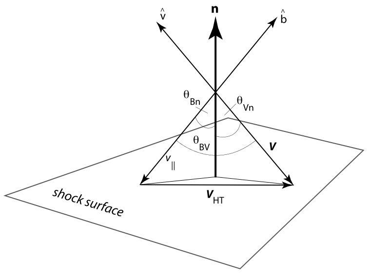
The de Hoffmann-Teller velocity is the same to both sides of the shock ramp, because of the continuity of normal component \(B_n\) and tangential electric field \(\mathbf{E}_t\). Thus, in the de Hoffmann-Teller frame there is no induction electric field \(\mathbf{E} = -\hat{n}\times\mathbf{U}\times\mathbf{B}\). The remaining problem is two-dimensional (because trivially \(\hat{n}\), \(\hat{b}\) and \(-v_\parallel\hat{b}\) are coplanar, which is nothing else but the coplanarity theorem holding under these undisturbed idealized conditions).
In the de Hoffmann-Teller (primed) frame the particle velocity is described by the motion along the magnetic field \(\hat{b}\) plus the gyromotion of the particle in the plane perpendicular to \(\hat{b}\): \[ \mathbf{v}^\prime(t) = v_\parallel^\prime\hat{b} + v_\perp\left[ \hat{x}\cos(\omega_{ci}t +\phi_0) \mp\hat{y}\sin(\omega_{ci}t + \phi_0) \right] \tag{21.25}\]
The unit vectors \(\hat{x}\), \(\hat{y}\) are along the orthogonal coordinates in the gyration plane of the ion, the phase \(\phi_0\) accounts for the initial gyro-phase of the ion, and \(\pm\) accounts for the direction of the upstream magnetic field being parallel (+) or antiparallel (-) to \(\hat{b}\).
In specular reflection (from a stationary shock) the upstream velocity component along \(\hat{n}\) is reversed, and hence (for cold ions) the velocity becomes (???) \[ \mathbf{v}^\prime = -v_\parallel^\prime\hat{b} + 2v_\parallel \cos\theta_{Bn}\hat{n} \] which (with \(\phi_0 = 0\)) yields for the components of the velocity \[ \frac{v_\parallel^\prime}{U} = \frac{\cos\theta_{Vn}}{\cos\theta_{Bn}}\left( 2\cos^2\theta_{Bn} - 1 \right) \quad \frac{v_\perp^\prime}{U} = 2\sin\theta_{Bn}\cos\theta_{Vn} \]
These expressions can be transformed back into the observer’s frame by using \(\mathbf{V}_\text{HT}\). It is, however, of greater interest to see under which conditions a reflected particle turns around in its upstream motion towards the shock. This happens when the upstream component of the velocity \(v_x = 0\) of the reflected ion vanishes. For this we need to integrate Equation 21.25 which for \(\phi_0 = 0\) yields \[ \mathbf{x}^\prime(t) = v_\parallel^\prime t \hat{b} + \frac{v_\perp}{\omega_{ci}}\left[ \hat{x}\sin\omega_{ci}t \pm\hat{y}(\cos\omega_{ci}t -1) \right] \]
Scalar multiplication with \(\hat{n}\) yields the ion displacement normal to the shock in upstream direction. The resulting expression \[ \mathbf{x}_n^\prime(t^\ast) = v_\parallel^\prime t \cos\theta_{Bn} + \frac{v_\perp}{\omega_{ci}}\sin\theta_{Bn}\sin\omega_{ci}t^\ast = 0 \tag{21.26}\] vanishes at time \(t^\ast\) when the ion re-encounters the shock with normal velocity \[ v_n(t^\ast) = v_\parallel^\prime \cos\theta_{Bn} + v_\perp\sin\theta_{Bn}\cos\omega_{ci}t^\ast \]
The maximum displacement away from the shock in normal direction is obtained when setting this velocity to zero, obtaining for the time \(t_m\) at maximum displacement (again including the initial phase here) \[ \omega_{ci}t_m + \phi_0 = \cos^{-1}\left( \frac{1 - 2\cos^2\theta_{Bn}}{2\sin^2\theta_{Bn}} \right) \tag{21.27}\]
This expression must be inserted in \(\mathbf{x}_n\) yielding for the distance a reflected ion with gyroradius \(r_{ci} = V/\omega_{ci}\) can achieve in upstream direction \[ \Delta x_n = r_{ci}\cos\theta_{Vn}\left[ (\omega_{ci}t_m + \phi_0)(2\cos^2\theta_{Bn} - 1) + 2\sin^2\theta_{Bn}\sin(\omega_{ci}t_m +\phi_0) \right] \tag{21.28}\]
For a perpendicular shock \(\theta_{Bn} = 90^\circ\) and \(\phi_0 = 0\) this distance is \(\Delta x_n \simeq 0.7 r_{ci} \cos\theta{Vn}\), less than an ion gyro radius. The distance depends on the shock normal angle, decreasing for non-planar shocks. Note that the argument of \(\cos^{-1}\) in Equation 21.27 changes sign for \(\theta_{Bn} \le 45^\circ\). Equation 21.26 has solutions for positive upstream turning distances only for shock normal angles \(\theta_{Bn} > 45^\circ\), for an initial particle phase \(\phi_0 = 0\).10 Reflected ions can return to the shock in one gyration time only when the magnetic field makes an angle with the shock normal that is larger than this value. For less inclined shock normal angles the reflected ions escape along the magnetic field upstream of the shock and do not return within one gyration. This sharp distinction between shock normal angles \(\theta_{Bn} < 45^\circ\) and \(\theta_{Bn} > 45^\circ\) thus provides the natural (kinematic specular) discrimination between quasi-perpendicular and quasi-parallel (planar) shocks we were looking for.
The theory of shock particle reflection holds, in this form, only for cold ions, which implies complete neglect of any velocity dispersion and proper gyration of the ions. The ions are considered of just moving all with one and the same oblique flow velocity \(\mathbf{U}\). In a warm plasma each particle has a different speed, and it is only the group of bulk velocity ions which are described by the above theory. Fortunately, these are the particles which experience the reflecting shock potential strongest and are most vulnerable to specular reflection. When temperature effects will be included, the theory is more involved in a number of ways:
- The de-Hoffmann-Teller velocity must be redefined to include the microscopic particle motion.
- The assumption of ideal specular reflection becomes questionable, as the particles themselves become involved into the generation of the shock potential. However, observations in space suggest that, for high flow velocities and supercritical Mach numbers, the simple kinematic reflection is a sufficiently well justified mechanism.
The formal treatment for warm ions are shown in P153 of Balogh and Treumann (2013). The result is that including thermal effect may
- modify the angle of transition, and
- will substantially affect the distance up to that a specularly reflected particle at the quasi-perpendicular shock can penetrate the upstream flow, i.e. it affects the width of the quasi-perpendicular shock-foot, even in the case when the reflection process is genuinely specular.
21.4.2 Foot Formation and Acceleration
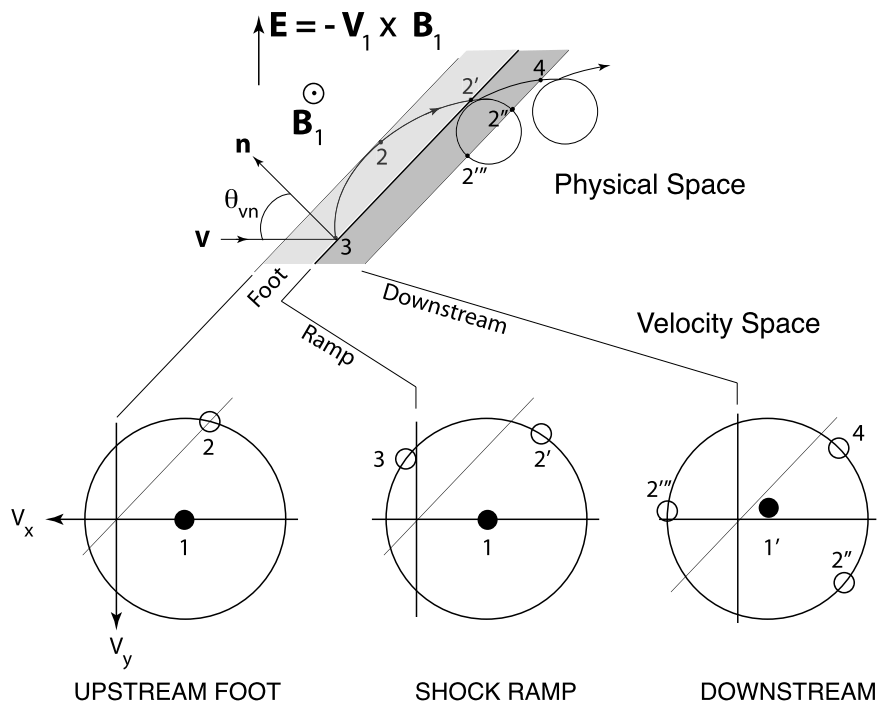
Shock reflected ions in a quasi-perpendicular shock cannot escape far upstream (see Figure 21.7). Their penetration into the upstream plasma is severely restricted by Equation 21.28. Within this distance the ions perform a gyration orbit before returning to the shock.
Since the reflected ions are about at rest with respect to the inflowing plasma they are sensitive to the inductive convection electric field \(\mathbf{E} = -\mathbf{U}_1 \times \mathbf{B}_1\) behaving very similar to pick-up ions and becoming accelerated in the direction of this field to achieve a higher energy (Schwartz et al. 1983). When returning to the shock their maximum (minimum) achievable energy is \[ \epsilon_\text{max} = \frac{m_i}{2}\left[ (v_\parallel^\prime + V_\text{HT})^2 + (V_\text{HT} \pm v_\perp)^2 \right] \tag{21.29}\]
This energy is larger than their initial energy with that they have initially met the shock ramp and, under favourable conditions, they now might overcome the shock ramp potential and escape downstream. Otherwise, when becoming reflected again, they gain energy in a second round until having picked up sufficient energy for passing the shock ramp.
In addition to this energization of reflected ions which in the first place have not made it across the shock, the reflected ions when gyrating and being accelerated in the convection electric field constitute a current layer just in front of the shock ramp of current density \(J_y\sim e n_\text{i,refl} v_\text{y, refl}\) which gives rise to a foot magnetic field of magnitude \(B_\text{z, foot}\sim \mu_0 j_y \Delta x_n\). It is clear that this foot ion current, which is essentially a drift current in which only the reflected newly energized ion component participates, constitutes a source of free energy as it violates the energetic minimum state of the inflowing plasma in its frame. Being the source of free energy it can serve as a source for excitation of waves via which it will contribute to filling the lack of dissipation. However, in a quasi-perpendicular shock there are other sources of free energy as well which are not restricted to the foot region.
Figure 21.8 shows a sketch of some of the different free-energy sources and processes across the quasi-perpendicular shock. In addition to the shock-foot current and the presence of the fast cross-magnetic field ion beam there, the shock ramp is of finite thickness. It contains a charge separation electric field \(E_x\) which in the supercritical shock is strong enough to reflect the lower energy ions. In addition it accelerates electrons downstream thereby deforming the electron distribution function.
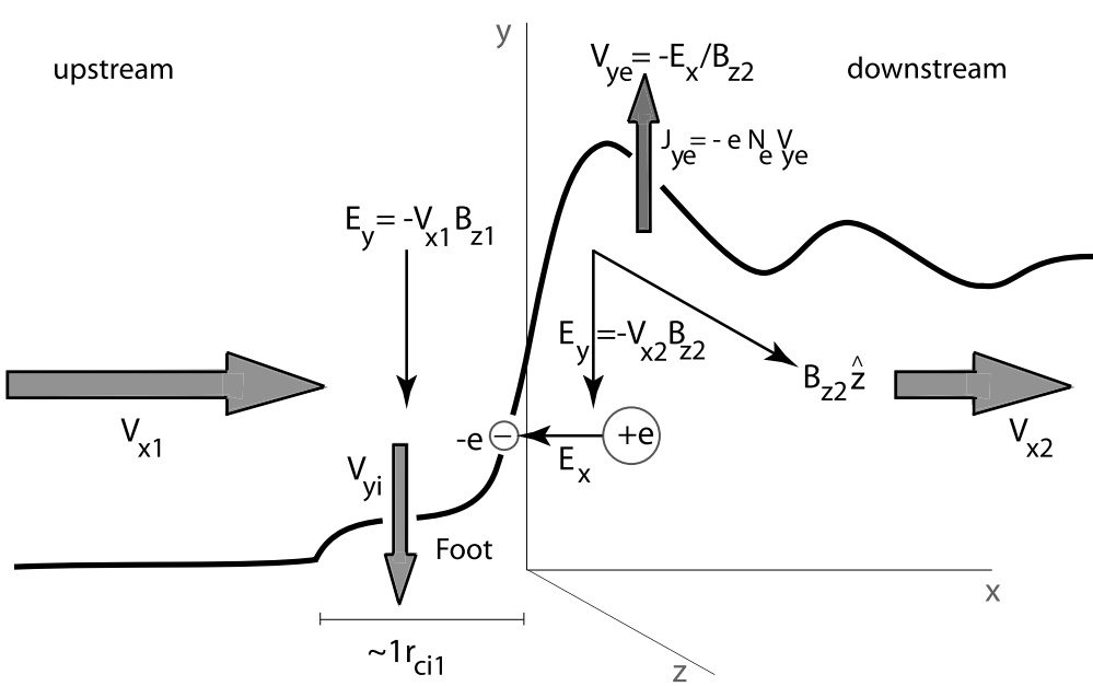
The presence of this field, which has a substantial component perpendicular to the magnetic field, implies that the magnetized electrons with their gyro-radii being smaller than the shock-ramp width experience an electric drift \(V_{ye} = -E_x/ B_{z2}\) along the shock in the ramp which can be quite substantial giving rise to an electron drift current \(J_{ye} = -en_\text{e,ramp}V_{ye} = en_\text{e,ramp}E_x/B_{z2}\) in the y-direction. This current has again its own contribution to the magnetic field, which at maximum is roughly given by \(B_z \sim \mu_0 J_{ye}\Delta x_n\). Here we use the width of the shock ramp. The electron current region might be narrower, of the order of the electron skin depth \(d_e = c/\omega_{pe}\). However, as long as we do not know the number of magnetized electrons which are involved into this current nor the width of the electric field region (which must be less than an ion gyro-radius because of ambipolar effects) the above estimate is good enough.
The magnetic field of the electron drift current causes an overshoot in the magnetic field in the shock ramp on the downstream side and a depletion of the field on the upstream side contributing to the steepness of the ramp. When this current becomes strong it contributes to current-driven cross-field instabilities like the modified two-stream instability.
Finally, the mutual interaction of the different particle populations present in the shock at its ramp and behind provide other sources of free energy. A wealth of instabilities and waves is thus expected to be generated inside the shock. To these micro-instabilities add the longer wavelength instabilities which are caused by the plasma and field gradients in this region. These are usually believed to be less important as the crossing time of the shock is shorter than their growth time. However, some of them propagate along the shock and have therefore substantial time to grow and modify the shock profile. In the following we will turn to the discussion of numerical investigations of some of these processes reviewing their current state and provide comparison with observations.
21.4.3 Shock Potential Drop
One of the important shock parameters is the electric potential drop across the shock ramp – or if it exists also across the shock foot. This potential drop is not necessarily a constant but changes with location along the shock normal. We have already noted that it is due to the different dynamical responses of the inflowing ions and electrons over the scale of the foot and ramp regions. Its theoretical determination is difficult, however when going to the de Hoffmann-Teller frame the bulk motion of the particles is only along the magnetic field, and in the stationary electron equation of motion the \(\mathbf{V}_e \times \mathbf{B}\)-term drops out and, to first approximation, the cross shock potential is given by the pressure gradient (when neglecting any contributions from wave fields). The expression is then simply \[ \Delta \Phi(x) = \int_0^x \frac{1}{eN_e(n)}\left[ \nabla\cdot \overleftarrow{P}_e(n) \right]\mathrm{d}\mathbf{n} \tag{21.30}\]
Integration is over \(n\) along the shock normal \(\hat{n}\). For a gyrotropic electron pressure, valid for length scales longer than an electron gyroradius, \(\overleftrightarrow{P}_e = P_{e\perp}\mathbf{I} + (P_{e\parallel} - P_{e\perp})\mathbf{B}\mathbf{B}/BB\) one obtains (Goodrich and Scudder 1984), taking into account that \(\mathbf{E}\cdot\mathbf{B}\) is invariant, \[ \frac{\mathrm{d}}{\mathrm{d}n}\phi(n) = -\frac{E_\parallel}{\cos\theta_{Bn}} = \frac{1}{eN_e}\left[ \frac{\mathrm{d}}{\mathrm{d}n}P_{e\parallel} - (P_{e\parallel} - P_{e\perp})\frac{\mathrm{d}}{\mathrm{d}n}(\ln B) \right] \] which, when used in the above expression, yields \[ e\Delta \Phi(x) = \int_0^x \mathrm{d}n\left\{ \frac{\mathrm{d}T_{e\parallel}}{\mathrm{d}n} + T_{e\parallel}\frac{\mathrm{d}}{\mathrm{d}n}\ln\left[ \frac{N(n)}{N_1}\frac{B_1}{B(n)} \right] + T_{e\perp}\frac{\mathrm{d}}{\mathrm{d}n}\ln\left[ \frac{B(n)}{B_1} \right] \right\} \]
This expression can approximately be written in terms of the gradient in the electron magnetic moment \(\mu_e = T_{e\perp}/B\) as follows: \[ e\Delta\Phi(x) \simeq \Delta(T_{e\parallel} + T_{e\perp}) - \int_0^x \mathrm{d}n \frac{\mathrm{d}\mu_e(n)}{\mathrm{d}n}B(n) \] with \(T_e\) in energy units. When the electron magnetic moment is conserved, the last term disappears, yielding a simple relation for the potential drop \(e\Delta\Phi(x) \simeq \Delta(T_{e\parallel} + T_{e\perp})\) as the sum of the changes in electron temperature. The perpendicular temperature change can be expressed as \(\Delta T_{e\perp} = T_{e\perp,1}\Delta B/B_1\) which is in terms of the compression of the magnetic field. Non-adiabatic effects contribute via the dropped integral term, which breaks the adiabatic invariant.
The parallel change in temperature is more difficult to express. One could express it in terms of the temperature anisotropy \(A_e = T_{e\parallel} /T_{e\perp}\) as has been done by Kuncic et al [2002], and then vary \(A_e\). But this depends on the particular model. It is more important to note that this adiabatic estimate of the potential drop does not account for any dynamical process which generates waves and substructures in the shock. It thus gives only a hint on the order of magnitude of the potential drop across the foot-ramp region in quasi-perpendicular shocks.
21.4.4 Shock Structure
Figure 21.9 shows observations from one of the first unambiguous satellite crossings of a quasi-perpendicular supercritical (magnetosonic Mach number \(M_\text{ms} \sim 4.2\)) shock at the Earth’s bow shock.
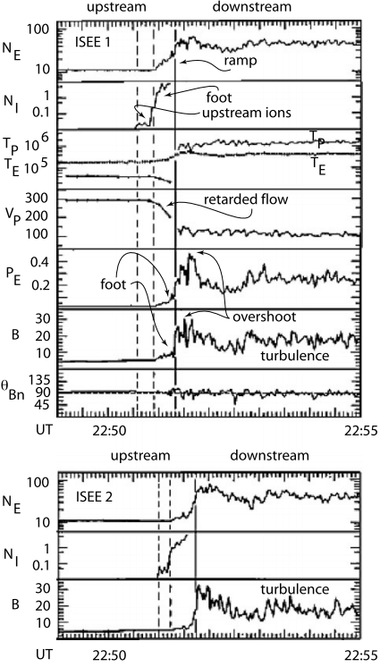
21.4.4.1 Observational evidence
The crossing occurred on an inbound path of the two spacecraft ISEE 1 (upper block of the figure) and ISEE 2 (lower block of the figure) from upstream to downstream in short sequence only minutes apart. In spite of some differences occurring on the short time scale the two shock crossings are about identical, identifying the main shock transition as a spatial and not as a temporal structure. Temporal variations are nevertheless visible on the scale of a fraction of a minute.
In this case, \(\theta_{Bn}\) is close to \(90^\circ\) prior to shock crossing (in the average \(\theta_{Bn} \sim 85^\circ\)), and fluctuates afterwards around \(90^\circ\) identifying the shock as quasi-perpendicular. Accordingly, the shock develops a foot in front of the shock ramp as can be seen from the slightly enhanced magnetic field after 22:51 UT in ISEE 1 and similar in ISEE 2, and most interestingly also in the electron pressure. At the same time the bulk flow velocity starts decreasing already, as the result of interaction and retardation in the shock foot region. The foot is also visible in the electron density which increases throughout the foot region, indicating the presence of electrons which, as is suggested by the increase in pressure, must have been heated or accelerated.
The best indication of the presence of the foot is, however, the measurement of energetic ions (second panel from top). These ions are observed first some distance away from the shock but increase drastically in intensity when entering the foot. These are the shock-reflected ions which have been accelerated in the convection electric field in front of the shock ramp. Their occurrence before entrance into the foot is understood when realising that the shock is not perfectly perpendicular. Rather it is quasi-perpendicular such that part of the reflected ions having sufficiently large parallel upstream velocities can escape along the magnetic field a distance larger than the average upstream extension of the foot. For nearly perpendicular shocks, this percentage is small.
The shock ramp in Figure 21.9 is a steep wall in B and \(P_E\), respectively. The electron temperature \(T_E\) increases only moderately across the shock while the ion temperature \(T_P\) jumps up by more than one magnitude, exceeding \(T_E\) downstream behind the shock. This behaviour is due to the accelerated returning foot-ions which pass the shock. \(P_E\), \(B\), and \(N_E\) exhibit overshoots behind the shock ramp proper. Farther away from the shock they merge into the highly fluctuating state of lesser density, pressure, and magnetic field that can be described as some kind of turbulence. Clearly, this region is strongly affected by the presence of the shock which forms one of its boundaries, the other boundary being the obstacle (Earth) which is the main responsible for the formation of the shock.
The evidence provided by the described measurements suggests that the quasi-perpendicular shock is a quasi-stationary entity. This should, however, not been taken apodictic. Stationarity depends on the spatial scales as well as the time scales. A shock is a very inhomogeneous subject containing all kinds of spatial scales; being stationary on one scale does not imply that it is stationary on another scale. For a shock like the Earth’s bow shock considered over times of days, weeks or years the shock is of course a stationary subject. However on shorter time scales of the order of flow transition times this may not be the case. A subcritical shock may well be stationary on long and short time scales. However, for a supercritical shock the conditions for forming a stationary state are quite subtle. From a single spacecraft passage like that described above it cannot be concluded to what extent, i.e. on which time scale and on which spatial scale and under which external conditions (Mach number, angle, shock potential, plasma-β,…) the observed shock can be considered to be stationary (a discussion of the various scales has been given, e.g, by Galeev et al, 1988). Comparison between the two ISEE spacecraft already shows that the small-scale details as have been detected by both spacecraft are very different. This suggests that – in this case – on time scales less than a minute variations in the shock structure must be expected.
Generally spoken, one must be prepared to consider the shock locally (on the ion gyroscale) and temporarily (on the ion-cyclotron frequency scale) as a non-stationary phenomenon (this has been realised first by Morse et al, 1972) which depends on many competing processes and, most important though only secondarily related to non-stationarity, a shock as a whole is not in thermal equilibrium. It needs to be driven by some energy source external to the shock in order to be maintained. It will thus be very sensitive to small changes in the external parameters and will permanently try to escape the non-equilibrium state and to approach equilibrium. Since its non-equilibrium is maintained by the conditions in the flow, it is these conditions which determine the time scales over which a shock evolves, re-evolves and changes its state. Real supercritical shocks, whether quasi-perpendicular or quasi-parallel, are in a permanently evolving state and thus are intrinsically nonstationary.
21.4.4.2 Simulation studies
Perpendicular or quasi-perpendicular collisionless shocks are relatively easy to treat in numerical simulations. Already from the first one-dimensional numerical experiments on collisionless shocks it became clear that such shocks have a very particular structure. This structure, which we have describe in simplified version in Figure 21.8 and which could to some extent also be inferred from the observations of Figure 21.9, becomes ever more pronounced the more refined the resolution becomes and the better the shorter scales can be resolved.
As already mentioned, collisionless shocks are in thermodynamic non-equilibrium and therefore can only evolve if a free energy source exists and if the processes are violent enough to build up and maintain a shock. Usually in a freely evolving system the free energy causes fluctuations which serve dissipating and redistributing the free energy towards thermodynamic and thermal equilibria. Thermal equilibria are characterised by equal temperatures among the different components, e.g. \(T_e = T_i\) which is clearly not given in the vicinity of a shock as seen from Figure 21.9. Thermodynamic equilibria are characterized by Gaussian distributions for all components of the plasma. To check this requires information about the phase space distribution of particles. Shocks contain many differing particle distributions, heated, top-flat, beam distributions, long energetic tails, and truncated as well as gyrating distributions which we will encounter later. Consequently, they are far from thermodynamic equilibrium.
For a shock to evolve the amount of free energy needed to dissipate is so large that fluctuations are unable to exercise their duty. This happens at large Mach numbers. The shock itself takes over the duty of providing dissipation. It does it in providing all kinds of scales such short that a multitude of dissipative processes can set on.
Scales
For a quasi-perpendicular shock propagating and evolving in a high-β plasma there is a hierarchy of such scales available. The kinetic \(\beta_{\text{kin}\perp} = 2\mu_0 N m_i V_n^2/2B^2 \equiv M^2 > 1\) implies that the kinetic energy in the flow exceeds the magnetic energy. Hence the flow dominates the magnetic field, which is transported by the flow. In plasmas with \(\beta_{\text{kin}\perp} = M^2 < 1\) the magnetic field dominates the dynamics, and shock waves perpendicular to the magnetic field cannot evolve. Parallel shocks are basically electrostatic in the \(\beta_{\text{kin}\perp}\gg 1\)-case and can evolve when the flow is sufficiently fast along the field, as is observed in the auroral magnetospheres of the magnetised planets in the heliosphere. On the other hand, for large Mach numbers and \(\beta \ge 1\) conditions shocks do exist, as the example of the solar wind shows.
The different scales can be organized with respect to the different regions of the shock.
The macroscopic scale of the foot region, which determines the width of the foot, is the ion gyroradius based on the inflow velocity \(r_\text{ci,1} = V_1/\omega_\text{ci,1}\). With the slight modification of replacing the upstream magnetic field with the (inhomogeneous) ramp magnetic field \(B_\text{r}(x)\) this also becomes approximately the scale of the macroscopic electric potential drop in the ramp, \(\Delta_{\phi, r}\sim r_\text{ci, r}\sim V_1 / \omega_\text{ci,r}\). This is an important difference which can be taken as a golden rule for estimates of the structure of quasi-perpendicular shocks even though, of course, these values are dynamical values which change from position to position across the foot and ramp. Observation evidence from the CLUSTER satellites are given in (Bale et al. 2003).
The ion inertial length \(d_i = c/\omega_\text{pi}\), which is also a function of space inside the ramp because of the steep density increase \(N(x)\). It determines the dispersive properties of the fast magnetosonic wave which is locally responsible for steeping and shock ramp formation.
The thermal ion gyroradius \(r_\text{ci} = v_\text{th,i}/\omega_\text{ci}\). It determines the transition from unmagnetized to magnetized ions and from non-adiabatic to adiabatic heating of the ions.
The density gradient scale \(L_P = (\nabla_x \ln P)^{-1}\). It determines the importance of drift waves along the shock which, when excited, structure the shock in the third dimension perpendicular to the shock normal and the magnetic field.
The electron inertial length \(d_e = c/\omega_{pe}\). It is the scale length of whistlers which are excited in front of the shock and are generally believed to play an essential role in shock dynamics.
The thermal electron gyroradius \(r_\text{ce} = v_\text{th,e}/\omega_\text{ce}\). It determines whether electrons behave magnetized or non-magnetized. In the shock they are usually magnetized under all conditions of interest. However, when non-adiabatic heating becomes important for electrons it takes place on scales comparable to \(r_\text{ce}\).
The Debye length \(\lambda_\text{D}\). It determines the dispersive properties of ion acoustic waves which are responsible for anomalous resistivity and for smaller scale density substructures in the shock like the phase space holes which evolve on scales of several Debye lengths. It also determines the scales of the Buneman two-stream (BTS) and modified two-stream (MTS) instabilities which are the two most important instabilities in the shock foot.
The importance of some of these scales has been discussed by Kennel et al. (1985) assuming that some mostly anomalous resistance has been generated in the plasma. In this case the speed of the fast magnetosonic wave, which is responsible for fast shock formation, is written as \[ c_\text{ms}^2 = c_\text{ia}^2 + \frac{V_A^2}{1+ k^2 R^2},\quad R = \begin{cases} R_\eta=(\eta / \mu_0)(k/\omega) & \eta \neq 0 \\ d_e=c/\omega_{pe} & \eta \to 0 \end{cases} \] taking explicitly care of the dispersion of the wave which leads to wave steeping. The macroscopic scale of shock formation enters here through the definition of \(R\) which in the collisionless case becomes the electron skin depth. Starting from infinity far away from the shock one seeks for growing solutions of the linear magnetic disturbance \(b_z \sim \exp \lambda_x\) in the stationary point equation \[ R_e^2 b_z^{''} + R_\eta b_z^{'} = D b_z,\quad D \equiv \frac{1 - M^2}{1 - c_\text{ia}^2 / V^2} \] where the prime \(' \equiv \partial/\partial x\) indicates derivation with respect to x. With \(b_z \to 0\) for \(x \to -\infty\) this yields for the spatial growth rate \[ \lambda_> = -\frac{R_\eta}{2d_e^2} + \left[ \frac{D}{d_e^2} + \left( \frac{R_\eta}{2d_e^2} \right)^2 \right]^{1/2} \to \frac{D^{1/2}}{d_e}\quad\text{for}\quad R_\eta \ll d_e \] which identifies the approximate shock transition scale as proportional to the electron skin depth, \(\Delta \simeq c / \omega_{pe}D^{1/2}\), just what one intuitively would believe to happen for freely moving electrons and ions. Since the upstream sound speed \(c_\text{ia} \ll V\) is small compared with the fast flow \(V\), we have \(D ≈ 1 - M^{-2}\), and the shock ramp width becomes slightly larger than the electron skin depth \(d_e = c/\omega_{pe}\), viz. \[ \Delta \simeq M(M^2 -1)^{-1/2}d_e \]
For large Mach numbers this width approaches \(d_e\). However, we have already seen that at large Mach numbers the competition between dispersion and dissipation does not hold anymore in this simple way.
With increasing wave number k the fast magnetosonic mode merges into the whistler branch with its convex dispersion curve. This implies that dispersive whistler waves will outrun the shock becoming precursors of the shock. Whistlers propagate only outside their resonance cone. The limiting angle between k and the magnetic field B for which the whistler outruns the shock is given by \(\theta_\text{wh,lim} \le \cos^{-1}[M_A(m_e/m_i)^{1/2}]\), artificially limiting the Alfvén Mach number \(M_A = V/V_A < 43\). A linear whistler wave precursor can stand in front of the quasi-perpendicular shock as long as the Mach number \(M < M_\text{wh}\) is smaller than the critical whistler Mach number
\[ \begin{aligned} M_\text{wh} &= \frac{1}{2}\left(\frac{m_i}{m_e} \right)^{1/2}|\cos\theta_{Bn}|\quad&\text{linear case} \\ M_\text{wh,nl} &= M_\text{wh}\sqrt{2}\left[ 1 - \frac{27\beta}{128 M_\text{wh}}^{1/3} \right]\quad&\text{nonlinear case} \end{aligned} \] The second expression results when including the nonlinear growth of the whistler amplitude during the steeping process [for the derivation of this expression see, e.g., Kazantsev, 1961; Krasnoselskikh et al, 2002].
In 1D simulations with all quantities changing only along the shock normal \(\hat{n}\) and the \(\mathbf{k}\)-vectors of waves along \(\hat{n}\) as well, one choses angles between \((\mathbf{k},\hat{n})\) and \(\mathbf{B}\) larger than this in order to have clean effects which are not polluted by those whistlers. However, the maximum phase speed of whistlers does not exceed the Alfvén speed by much. Hence, as long as the upstream velocity is less than this maximum whistler speed, a standing whistler precursor will be attached to the shock in front. When the upstream velocity exceeds this velocity, phase standing whistlers become impossible. This happens at the critical whistler Mach number. The shock structure becomes more complicated then by forming shock substructures [Galeev+, 1988] on scales of \(d_e = c/\omega_{ce}\), and the shock might become non-stationary [Krasnoselskikh+, 2002].
1D Structure
One-dimensional observations as those presented in Figure 21.9 confirm the theoretical prediction of the gross structure of a quasi-perpendicular shock. Observations are possibly limited by not resolving the spatial structure of the shock on smaller scales and the lack of inference about the evolution of the shock. To achieve a clearer picture of both the structure and the evolution, the observations must be supported by numerical simulations.
The Shock Transition Scale
The width of the shock transition is particularly important in its relation to the width of the electrostatic potential drop across the shock. There are essentially three transition scales: the magnetic scale \(\Delta B\), the density scale \(\Delta N\), and the electric potential scale \(\Delta E\). Since the shock is not in pressure equilibrium, the first two scales are not necessarily be proportional to each other. However, the electric field and density gradient might be related, so one expects that \(\Delta N\,\sim\,\Delta E\) even though this is not necessarily so, in particular not when instabilities arise which cause very small scale electric field radients. In principle one can distinguish three different cases [Lembege et al, 1999] which describe different physics:
\(\Delta E \gg \Delta B\). This is a case that has been reported to have been observed in Bow shock crossings. The magnetic ramp is much steeper in this case than the structure of the electric field. The latter smears out over the foot and ramp regions. In this case the electrons will behave adiabatically, while the ions may be only partially or even non-magnetized.
\(\Delta E \sim \Delta B\). In this case there will be a significant deviation from adiabatic behavior of the electrons in the shock transition. Electron heating and motion will not be adiabatic anymore, and the electron distribution will significantly be disturbed.
\(\Delta E \ll \Delta B\). This case which is also called the ‘isomagnetic’ transition [Eselevich, 1982; Kennel et al, 1985] corresponds to shock transitions with electrostatic substructuring which are sometimes also called subshocks.
The generation of these quasi-perpendicular shock structures by a variety of instabilities might even turn the shock foot and ramp regions into regions where large anomalous collisions and thus resistances are generated as the result of wave-particle interactions. In this case the shock returns to become resistive again due to preventing large numbers of reflected ions from passing across the steep shock ramp and large shock potential, using the kinetic energy of the reflected particle population for the generation of a broad wave spectrum which acts to scatter the particles around in the foot and ramp regions and, possibly, also up to some distance in the transition region behind the ramp. This kind of confinement of reflected particles over long times will then be sufficiently long for providing the heating and dissipation which is required for sustaining a resistive shock which, then, is the result of the combined action of ion viscosity and anomalous resistivity, i.e. anomalous collisions. In addition, the scattering of the trapped reflected particle population necessarily results in plasma heating, and some particles will become accelerated to high velocities in these interactions as well. It is then possible that these particles provide the seed population for energetic particles which have been accelerated to high energies in the well-known shock-Fermi-one and shock-Fermi-two acceleration mechanisms.
21.4.5 Shock Reformation
Supercritical shocks do under certain conditions reform themselves periodically – or quasi-periodically –, which is kind of a non-stationarity of the shock that does not destroy the shock but, at the contrary, keeps it intact in a temporarily changing way. We will come later to the problem of real non-stationarity.
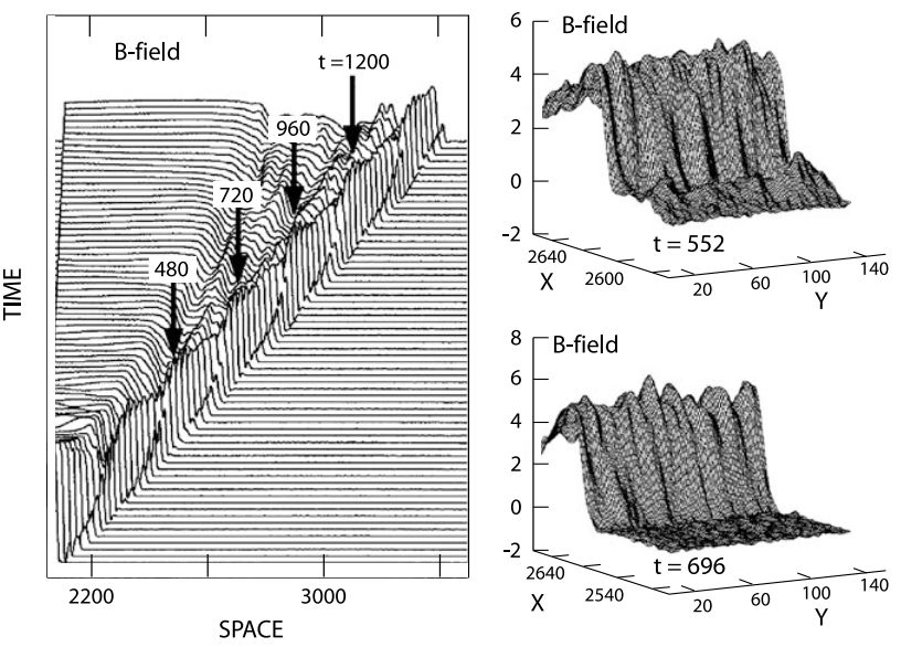
For illustration, Figure 21.10, on its left, shows a low mass-ratio example of the temporary evolution of a shock during shock reformation in a magnetic field stack plot. On its right the structure of the shock ramp at two different two reformation times is plotted along the shock ramp. There is a distinct reformation cycle in this simulation and also a distinct structure of the ramp/shock front in the tangential direction which is far from being smooth, a fact to which we will return during discussion of non-stationarity of shocks. The shock not only reforms cyclically in time, it also develops ripples along its surface which travel like waves along the shock.
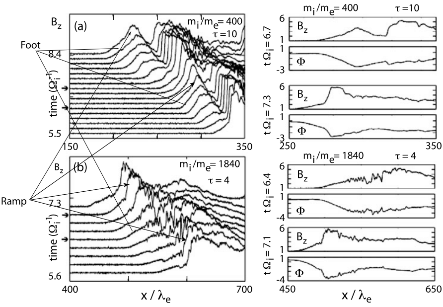
Full PIC simulations show that reformation at least occurs at small ion-\(\beta_i \sim 0.2\). In these simulations the shock is produced by injecting a uniform plasma from -x and letting it reflect from a stationary wall at the right end of the simulation box. The plasma carries a uniform magnetic field in the (x,z)-plane, and the plasma is continuously injected in the +x-direction.11 Since the right-hand reflecting boundary is stationary the shock, which is generated via the ion-ion beam instability in the interaction of the incoming and reflected ion beams, moves to the left at velocity given by the supercritical shock Mach number \(M_A \sim 4.5\). The upstream plasma has \(\beta_i = \beta_e = 0.05\), and the shock normal angle is \(\theta_{Bn} = 87^\circ\).
Two runs of these simulations are shown in Figure 21.11, one is for a mass ratio of 400, the other for a mass ratio of 1840. The left-hand side of the figure shows stack plots of time profiles of the nearly perpendicular magnetic field \(B_z\) with time running in equidistant units upward on the ordinate. Since the plasma is injected from the left and reflected at the right boundary the shock is seen to move from the right to the left. The magnetic profiles are strikingly similar for both mass ratios. In both cases a relatively flat foot develops in front of the steeper shock ramp caused by the shock reflected ions. The magnetic field of this foot starts itself increasing with time with growth being strongest close to the upstream edge of the foot until the foot field becomes so strong that it replaces the former shock ramp and itself becomes the new and displaced shock ramp.
This is seen most clearly in the upper low mass-ratio part of the figure. The foot takes over, steepens and becomes itself the shock. One can recognise in addition that, even earlier, the intense foot already had started reflecting ions by himself and developing its own flat pre-foot region. This pre-foot evolves readily to become the next foot, while the old ramps become part of the downstream turbulence.
The one-dimensional full particle PIC simulations by Umeda and Yamazaki (2006) at Mach number \(M_A = 10\) and medium mass ratio \(m_i/m_e = 100\) throw additional light on the reformation process when keeping in mind that reformation is not as strongly dependent on the mass ratio as originally believed. Figure 21.12 shows a collection of their results which this time are represented in the shock frame of reference.
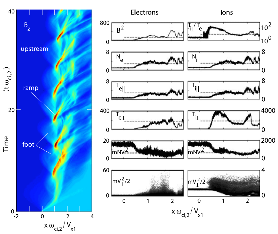
The simulations have been performed by assuming an initial Rankine-Hugoniot equilibrium in the PIC code. The non-physicality of this initialisation is manifested in the initial evolution over the first few ion cyclotron periods. During this time the simulation adjusts itself to the correct physics, and the non-physical disturbance decays. The shock frame has shifted by this to a new position, which in the shock frame is located farther downstream (which takes into account of the moment transferred to the shock by the reflection of the upstream ions who lower the shock speed).
The further evolution of the shock shows the quasi-periodic reformation and the play between the foot and the ramp formation. The periodicity is roughly \(\sim 6 \omega_{ci,\text{down}}^{-1} \sim T_{i,\text{down}}\). When the foot takes over to become the ramp, the ramp jumps ahead in a fraction of this time. Afterwards the formation of the foot retards the ramp motion, and the ramp softens and displaces itself downstream to become a downstream moving spectrum of magnetic oscillations which is injected into the downstream region in the form of wave packets. The various plasma parameters in the left part of the figure show in addition the compression of plasma and field, and the dominance of perpendicular ion heating which is, of course, due to the accelerated foot ions which pass into downstream.
21.4.6 Ion Dynamics
21.4.6.1 Ion Dynamics in Shock Reformation
Reflected particles are forming a foot on the perpendicular shock and may contribute to the reformation of the shock.
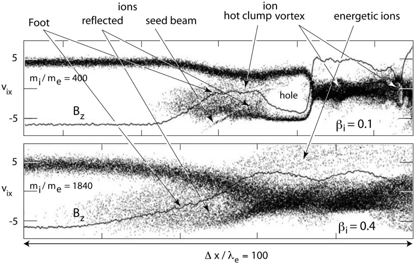
Figure 21.13 shows the ion phase space plots for the two mass ratios \(m_i/m_e = 400\) (top) and 1840 (bottom) respectively. Both plots show just the enlarged shock foot transition region over the same scale of \(100 d_e\). The electron \(\beta_e = 0.2\) has been kept constant in both simulations, while the ion \(\beta_i\) has been changed. Only the normal component of the ion velocity is shown for the nearly perpendicular supercritical shock. In both plots the magnetic field \(B_z\) has been drawn as a thin continuous line showing the magnetic shock profile over the spatial distance \(\Delta x\).
The upper (low-mass-ratio) low-\(\beta_i\) panel shows the cold dense ion inflow at velocity \(v_{ix} \sim 5\) (in units of the upstream Alfvén velocity) being retarded to nearly Mach number 1 already when entering the foot. This retardation is due to its interaction with the intense but cold (narrow in velocity space) reflected ion beam which is seen as the narrow negative \(v_{xi}\)-velocity beam originating from the shock ramp. This reflected ion beam needs a certain distance to interact with the upstream plasma inflow. This distance is the length the beam-beam excited waves need to grow. But once the interaction becomes strong enough, the reflected ions are scattered by the waves into a hot ion clump in addition to being turned around by gyration. Both effects cause a reduction in velocity vx of the reflected ions which, being accelerated by the convection electric field, turn to flow in y direction and cause the magnetic bump that develops in this region of the foot. It is interesting to remark that in the \((v_x, x)\)-plane the reflected ions close with the upstream flow into an hot ion ring distribution (vortex) just in front of the ramp of which the hot ion clump that brakes the inflow is the upstream boundary. Behind the ramp, which is the point of bifurcation of the ion distribution, i.e. the location where the reflection is at work, a broad hot ion distribution arises which at some locations shows rudimentary remains of ion vortices from former reformation cycles. Their magnetic signatures are the dips seen in the magnetic field. The next reformation cycle can be expected to completely close the ion vortex in the foot and to transform the ramp from its current position to the position of the foot. The first sign of this process is already seen in the foot ion distribution, which shows the birth of a faint new reflected ion beam at high negative speeds. This beam is not participating in the formation of the ring but serves as the seed of the newly reflected population.
The same behaviour is found in large mass ratio simulations as long as \(\beta_i\) is small. This is obvious from the large mass-ratio magnetic field shown in Figure 21.11. As long as \(\beta_i\) remains to be small, the shock undergoes reformations also for realistic mass ratios. In other words, as long as the plasma is relatively cool the real shocks found in nature should develop feet which at a later time quasi-periodically become the shock ramp.
This changes completely, when \(\beta_i\) increases as is suggested from consideration of the lower panel in Figure 21.13. There a realistic mass ratio has been assumed, but \(\beta_i = 0.4\), and no reformation is observed, at least not during the realisable simulation times. Instead, the shock develops a very long foot region that is extended twice as far into the upstream region as in the low-\(\beta_i\) case. Clearly, the high ion temperature smears out the reflected ion population over the entire gap region between the upstream and reflected beam regions, and no vortex can develop. This implies that the foot remains smooth and does not evolve into a ramp.
However, inspecting the panels of Figure 21.13 it becomes immediately clear that suppression of reformation is a relative process. Reformation will be suppressed only when the thermal speed \(v_\text{th,i}\) of the ions is large enough to bridge the gap between the reflected and incoming ion beams, i.e. large enough to fill the hole. Semi-empirically one can establish a condition for shock reformation as \(v_i < \alpha V_{n1}\) when taking into account that the normal speed of incoming ions is simply specularly turned negative. Since this is never exactly the case, the coefficient will roughly be in the interval \(1.5 < \alpha < 2\). This condition for reformation to occur can be written as \[ M_A > \frac{\beta_i^{1/2}}{\alpha} \tag{21.31}\] where the Alfvén Mach number is defined on \(V_{1n}\). The larger the Mach number becomes the less suppression of reformation will play a role, and at high Mach numbers one expects that either reformation becomes a normal process or that other time-dependent processes set on which lead to a non-stationary state where the shock reformation becomes a chaotic and unpredictable process. As we have argued earlier this is quite normal as the shock is thermodynamically and thermally in a non-equilibrium state: it is a region where electrons and ions have violently different temperatures; it is not in pressure equilibrium; upstream and downstream temperatures are different; and it hosts a number of non-Maxwellian phase space distributions all concentrated in a small volume of real space.
21.4.6.2 Ion instabilities and ion waves in the foot and ramp region
From the field and particle properties demonstrated in simulations of quasi-perpendicular supercritical shocks, it has become obvious that in the different regions of the shock transition the particle distributions carry free energy. This is true for the foot region, the shock transition and overshoot as well as the downstream region. And it is true for both species, electrons and ions. This free energy is the source of a number of instabilities which excite waves of different kinds in the various shock transition regions which can be measured.
The instabilities are not primarily driven by temperature anisotropy, but rather by differences in bulk flow properties of the different species. We therefore ignore the temperature anisotropy differences even though such instabilities may arise, in particular when ion-whistlers can be excited by temperature anisotropy. To some extent the occurrence of two (counter-streaming in the x-direction of shock normal) ion beams already fakes a bulk temperature on the ion component thus generating some relationship between a two-beam situation and a temperature anisotropy. Similarly transversely heated reflected ions superposed on a low perpendicular temperature inflowing ion background fakes a perpendicular temperature anisotropy. For our purposes, however, the bulk flow differences are more interesting and have, in fact, been more closely investigated right from the beginning.
Let us first consider the foot region. The free energy sources here are the relative drifts between the incoming electrons and reflected ions and the incoming electrons and incoming ions. The presence of the reflected ions causes a decrease of the ion bulk velocity in the foot region. This implies that the incoming electrons are decelerated so that the current in shock normal direction is zero, i.e. the flow is current-free in normal direction. However, this has the consequence that a relative bulk velocity between electrons and reflected ions or electrons and incoming ions arises. These differences will contribute to the excitation of instabilities. In this section we will restrict to ion instabilities leaving the essentially more interesting ion-electron instabilities for the next section. A list of the most important instabilities in the foot region is given in Table 21.2. It is interesting to note that only a few of these instabilities have ever been identified in actual observations and in the simulations even though theoretically they should be present. This can have several reasons, too small growth rates, too strong Landau damping, for instance, in the presence of hot ions, convective losses or very quick saturation due to heating effects, competition with other waves or wave-wave interaction and so on.
The most relevant instabilities generated in the shock foot have been identified as the whistler instability for nearly perpendicular supercritical but low-Mach number shocks, leading to foot formation but not being decisive for feet, as it has turned out that feet in this Mach number and shock-normal angle ranges are produced by accumulation of gyrating ions at the upward edge of the foot.
| Instability | Excitation by | Source of free energy | Direction of propagation |
|---|---|---|---|
| Ion-ion streaming instability | Reflected and transmitted ions | Relative streaming between the ion species | \(\theta_{kB} = 90^\circ\) |
| Kinetic cross-field streaming instability | Reflected ion | Relative streaming between the reflected ions and the solar wind electrons | \(\theta_{kB} \in (0^\circ, 90^\circ)\) |
| Kinetic cross-field streaming instability | Transmitted ion | Relative streaming between the transmitted ions and the electrons | \(\theta_{kB} \le 90^\circ\) |
| Lower-hybrid drift instability | Reflected ions | Relative cross-field drift between the reflected ions and the electrons; density gradient | \(\theta_{kB} < 90^\circ\) |
| Lower-hybrid drift instability | Drifting electrons | Relative cross-field drift between the reflected ions and the electrons; density gradient | \(\theta_{kB} < 90^\circ\) |
| Ion-acoustic instability | Transmitted ion | Relative streaming between the ion species and the electrons | \(\theta_{kB} < 90^\circ\) |
| Electron-cyclotron drift instability | Drifting electrons | Electron drift relative to the solar wind ions | \(\theta_{kB} \simeq 90^\circ\) |
| Whistler instability | Electrons | Electron thermal anisotropy \(T_{e\perp}> T_{e\parallel}\) | \(\theta_{kB} \simeq 0^\circ\) |
It is similar in the ramp region, with the fact that not all of these instabilities and waves are confirmed from neither observation nor simulation.
21.4.6.3 Downstream region
Detached shocks that evolve in front of blunt obstacles like a magnetosphere, in particular, possess extended downstream regions which separate the obstacle from the undisturbed upstream region. These regions are the domains of compressional waves – of the family of magnetosonic waves – with upstream directed phase and group velocities larger than the downstream flow velocity that in a characteristic flow time across the downstream distance from the shock to the obstacle can make it upstream to reach the shock, which forms the spatial envelope of these waves thereby confining them to downstream of the shock transition.
This is the fluid picture of the evolution of the region downstream of the shock. For a curved collisionless supercritical shock it is very difficult to distinguish between the processes triggered by the quasi-perpendicular and quasi-parallel parts separately. It is not until we discuss more about the quasi-parallel shock are we able to have a comprehensive description of the downstream region.
Collisionless shocks cannot be described solely in the fluid picture, however. Therefore the downstream region has quite a different behaviour from that inferred from the hydrodynamic description. This is particularly true for quasi-parallel shocks, but also for quasi-perpendicular shocks. Downstream of a quasi-perpendicular super-critical shock the conditions are as well very different from those which the fluid picture prescribes which of the plasma properties basically predicts an increase in the fluid pressure anisotropy due to compression of the magnetic field and plasma under conservation of the fluid magnetic moment (the ratio \(T_\perp/B\)), the deviation of the flow around the obstacle, draping of the magnetic field, and a pile-up region of the magnetic field close to the obstacle where pressure balance requires dilution of the plasma.
The main reasons for a deviation from this average and laminar behaviour of the downstream region are that in the supercritical case the fluid picture does not contain the ion (and electron) reflection processes and their consequences for shock foot formation, ramp physics and formation of the shock overshoot. Since collisional dissipation is out of question, the reflection mechanisms replace the necessary dissipation. It is easy to estimate, for instance for the quasi-perpendicular Earth’s bow shock, how much energy must be dissipated in order to adjust for the differences in the flow properties between upstream and downstream. For an upstream solar wind of nomial density \(n = 5\times 10^6\,\text{m}^{-3}\) and velocity \(V_1 = 500\,\text{km/s}\) at 1 AU, Mach number \(M_A = 5\) and moderate shock strength (compression ratio) of \(B_2 / B_1 = 3\), the energy density in the flow behind the shock (\(M_A = 1\)) is just half the energy density in the solar wind. Thus 50% of inflow energy must be dissipated by the shock. Since at most 10% of the ions are reflected (corresponding to 10% of incoming energy only), the remaining 40% are absorbed and dissipated in other ways.
A first simple effect that affects the region behind the shock ramp is that the reflected ions are accelerated by the motional electric field in the shock foot along the shock surface in the direction perpendicular to the upstream magnetic field to energies that are much higher than the kinetic energy of the incoming ions, thereby absorbing a substantial part of inflow energy. Acceleration of the 10% reflected ions by a factor 2 gives already 40% of energy dissipation. Hence this is the main dissipation mechanism. This acceleration affects the nearly periodic reformation of a quasi-perpendicular shock when these ions carry a drift current and gyrate at high speeds and large ion gyroradii in the upstream magnetic field. However, after a few such gyrations they have gained sufficient energy to break through the reflecting shock potential and overcome the shock barrier to enter the downstream flow region. Downstream of the quasi-perpendicular shock they appear as an energetic gyrating ion component with much larger perpendicular than parallel energy.
In fact these gyrating energetic ions have been observed (Sckopke et al. 1983). They are a source of free energy and excite a number of instabilities like electromagnetic ion-cyclotron waves which can grow to large amplitudes downstream of the shock and contribute to the magnetic fluctuation that are observed downstream. Even mirror modes just behind the shock have been reported [Czaykowska et al, 1998]. The rms amplitudes \(b_\text{rms} = \sqrt{|\mathbf{b}|^2} \sim B_2\) of these waves downstream of the shock are comparable to the average downstream field \(B_2\). Therefore these waves contribute to the energy balance. Moreover, since they are convected downstream and damp away, they contribute to heating of the downstream plasma and shock energy dissipation.
The larger amplitude waves do not damp but decay into other shorter amplitude waves or by ponderomotive force interaction may stabilise and form large amplitude localised magnetic structures, density pulses or also narrow current sheets. The physics of these structures is still barely understood. Sometimes one speaks about downstream turbulence which, however, is not qualified and also unjustified as turbulence can hardly develop in the downstream region because it has not sufficient time for reaching a well mixed state. This would require a very large extended region and relatively quiet boundary conditions with continuous inflow at an approximately constant energy level. It would also require stationarity of the shock which is definitely not given, as we will see later when discussing the problem of stationarity. Shock reformation is already kind of a rather non-stationary process that makes the development of downstream turbulence rather doubtful.
21.4.7 Electron Dynamics
Too complicated. Takes time to digest!
More important than whistlers have turned out the Buneman and modified two-stream modes, the former dominating shocks at perpendicular angles, the latter growing slowly but dominating at more oblique angles and at later simulation times with the effect of completely restructuring both the shock feet and ramps. Both instabilities generate phase space holes which during reformation survive and are added to the downstream plasma and, in addition, being responsible for low magnetic field values.
21.4.8 Stationarity
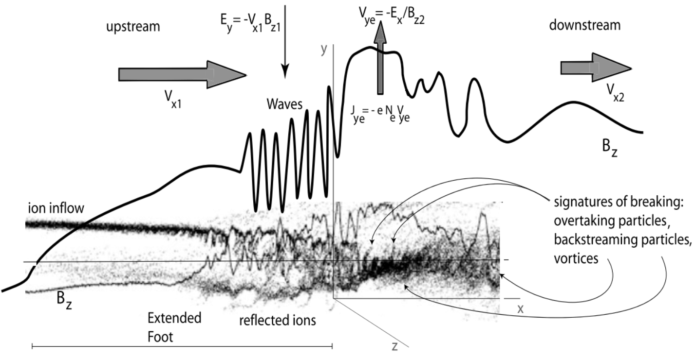
21.4.8.1 Formation of ripples
1D theory and 1D simulations implicitly treat the shock as an infinitely extended plane surface. In addition they allow only for instabilities to evolve in the direction of the shock normal at an angle relatively close to 90◦ such that any waves along the shock surface are completely excluded and waves parallel to the magnetic field have very small wave numbers \(k = k_x \cos\theta_{Bn} \ll k_x\) corresponding to very long parallel wavelengths. To be more realistic, 2D PIC simulations have been performed to investigate the effect of the additional freedom given by the second spatial dimension which allows instabilities to evolve in other than the shock normal direction.
3D PIC simulations of quasi-perpendicular shocks at a realistic mass ratio by Shinohara & Fujimoto [2010] found very strong wave activity in the shock foot region which is permitted by the inclusion of the third dimension. These waves cause a stronger then known upstream electron acceleration and the generation of non-thermal electrons.
The lesson learned is, however, quite simple: the shock exhibits structure along its surface which can presumably be attributed to waves running along the shock front and modulating it temporarily and spatially. There are at least three types of ripples: (1) short scale (below ion inertial length) lower-hybrid waves (typically about perpendicular to the magnetic field) supported by cross field currents instabilities [Lembège and Savoini, 1992], (2) longer scale (of the order of one or a few ion inertial lengths) oblique whistler waves (Hellinger et al. 2007; Lembège et al. 2009), and (3) even much longer “Alfvén wave” ripples (several ion inertial lengths) [Winske and Quest (1988); Saito and Umeda, 2011].
21.5 Supercritical Parallel Shock
From MHD or double adiabatic theory, parallel shocks are more special in that the magnetic field strength remains unchanged so the equations effectively describe pure gasdynamic solutions. Kuznetsov and Osin (2018) presents a simplified solution in a 1D parallel shock case with parallel and perpendicular thermal energy heat fluxes \(S_\parallel\) and \(S_\perp\) included. Note again the original CGL theory assumes 0 heat fluxes.
However, as have been indicated in Section 21.1.7, this does not cover the real physics involved into parallel shocks which must be treated on the basis of kinetic theory. These shocks possess an extended foreshock region with its own extremely interesting dynamics for both types of particles, electrons and ions, reaching from the foreshock boundaries to the deep interior of the foreshock. Based mostly on kinetic simulations, the foreshock is the region where dissipation of flow energy starts well before the flow arrives at the shock. This dissipation is caused by various instabilities excited by the interaction between the flow and the reflected particles that have escaped to upstream from the shock. Interaction between these waves and the reflected and accumulated particle component in the foreshock causes wave growth and steepening, formation of shocklets and pulsations and causes continuous reformation of the quasi-parallel shock that differs completely from quasi-perpendicular shock reformation. It is the main process of maintaining the quasi-parallel shock which by its nature principally turns out to be locally nonstationary and, in addition, on the small scale making the quasi-parallel shock close to becoming quasi-perpendicular for the electrons. This process can be defined as turbulent reformation, with transient phenonmena like hot flow anomalies, foreshock bubbles, and the generation of electromagnetic radiation.
The turbulent nature implies that the quasi-parallel shock transition is less sharp than the quasi-perpendicular shock transition and thus less well defined; there exists an extended turbulent foreshock instead of a shock foot. This foreshock consists of an electron and an ion foreshock. The main population is a diffuse ion component. The turbulence in the foreshock is generated by the reflected and accelerated foreshock particle populations. An important point in quasi-parallel shock physics is the reformation of the shock which works completely differently from quasi-perpendicular shocks; here it is provided by upstream low-frequency electromagnetic waves excited by the diffuse ion component. Steepening of these waves during shockward propagation and addition of the large amplitude waves at the shock transition reforms the shock front. The old shock front is expelled downstream where it causes downstream turbulence. During the reformation process the shock becomes locally quasi-perpendicular for the ions supporting particle reflection.
21.5.1 Basic Properties
In a quasi-parallel shock the combined geometries of the upstream magnetic field and generally curved shock surface prevent the shock-reflected particles from immediate return to the shock. The reason is that their gyro-orbits, after having suffered reflection from the shock ramp, lie completely upstream, outside the shock ramp, such that they do not touch the shock ramp again after reflection. Since, in addition, their upstream velocities have a large component parallel to the upstream magnetic field, which increases the more the shock-normal turns parallel to the upstream magnetic field, the reflected particles are enabled to escape upstream from the shock along the magnetic field thereby escaping backward convection and forming fast upstream particle beams.
A quasi-parallel supercritical collisionless shock thus populates the upstream space with a reflected particle component. This population moves a long distance away from the shock along the magnetic field. Was the upstream flow, in the case of the quasi-perpendicular shock, completely uninformed about the presence of the shock up to a distance of the mere width of the shock foot so, at the quasi-parallel shock, it receives a first signal of the presence of a shock already at quite a large upstream distance when the first and fastest reflected particles arrive on the magnetic field lines that connect the flow to the shock. It is, in fact, only these particles that can inform the flow about the presence of a supercritical shock, because any low-frequency plasma wave cannot propagate far upstream for supercritical Mach numbers \(M > M_c\), while any electromagnetic radiation that is generated at the shock has frequency \(\omega_\text{rad} > \omega_\text{pe}\). The upstream flow recognizes the reflected particles in its own frame of reference as a high-speed magnetic-field aligned beam. Thereby a beam-beam configuration is created which leads to a number of beam-driven instabilities. These excite various plasma waves that fill the space in front of the shock and modify its properties.
Figure 21.15 shows a sketch of the magnetic profile of a supercritical quasi-parallel shock which contrasts the profile of a quasi-perpendicular shock that has been given in Figure 21.8. The quasi-parallel magnetic shock profile is much stronger distorted than that of a quasi-perpendicular shock, such that it becomes difficult to identify the location of the genuine shock ramp on the profile.
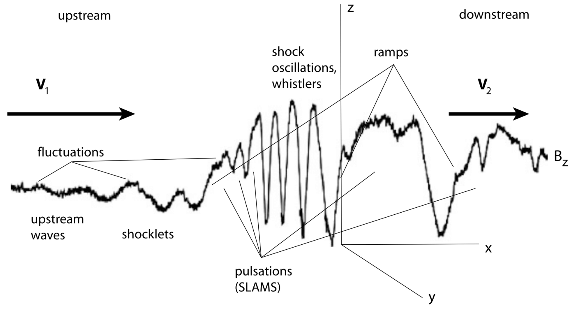
The main structural difference between quasi-perpendicular and quasi-parallel shocks is that quasi-perpendicular shocks possess a narrow \(\sim 1 r_\text{ci}\) wide foot region that is tangential to the shock surface, while quasi-parallel shocks possess an extended foreshock region. Interestingly, in curved shocks which arise, for instance, in front of spatially confined obstacles, both phases of a supercritical shock can coexists at the same time, being spatially adjacent to each other. An example is shown in Figure 22.14 in the sketch of the curved Earth’s bow shock. Dealing with quasi-parallel shocks means to a large extent dealing with the processes that are going on in the foreshock. It will thus be quite natural to start with a discussion of the properties of the foreshock.
However, before continuing we point out that in spite of the strict distinction between the quasi-perpendicular and quasi-parallel shocks there is also a close relation between the two. Both, being supercritical, can exist only because they reflect ions; and both possess an upstream region in front of the shock transition that is populated by the reflected ions. That this region is narrow in the case of quasi-perpendicular shocks is a question of the ions being tied to the magnetic field, which also holds in the case of the quasi-parallel shock. At quasi-perpendicular shocks the reflected ions do readily return to the shock. At the quasi-parallel shock they ultimately do also return to the shock, but only after having been processed far away from the shock in the foreshock, having coupled to the flow, having passed several stages in this processing, and having become the energetic component of the main flow. As such they finally arrive at the shock together with the stream. In between their main duty was to dissipate the excess energy, which they possessed when arriving for the first time at the shock and which could not be dissipated in the narrow shock-ramp transition region. This could been achieved only in the broad extended foreshock which, seen from this point of view, is already the shock. Therefore, the main physical difference between the quasi-perpendicular and quasi-parallel shocks is the dissipation processes.
21.5.2 Foreshock
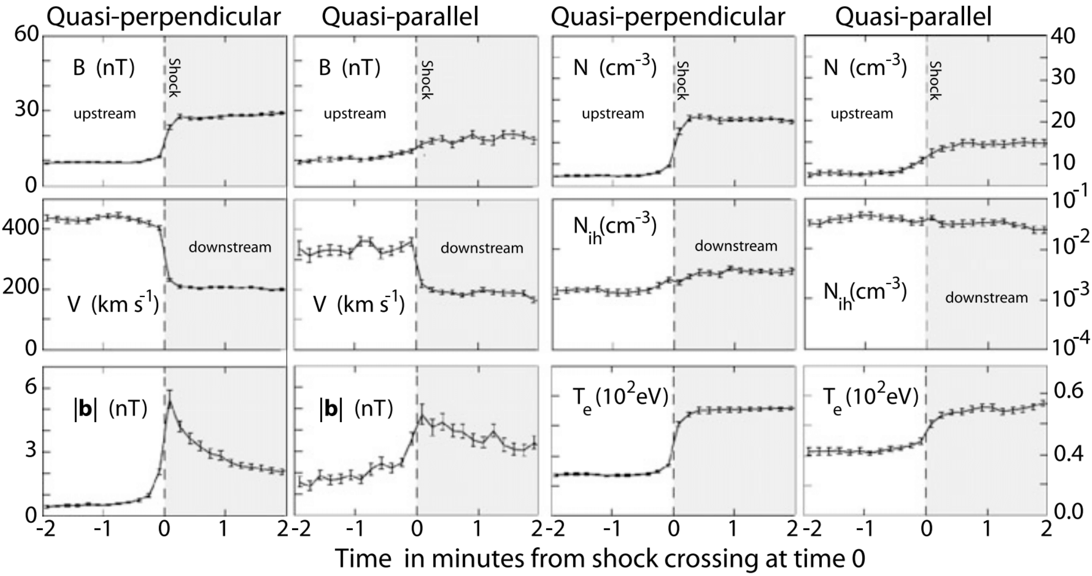
Figure 21.16 shows at one glance the main differences in the (average) bulk plasma parameters between quasi-perpendicular and quasi-parallel shocks as measured with the AMPTE IRM spacecraft at many crossings of the bow shock. The data used in this figure have been stapled, averaged and plotted with respect to the time normalised to the shock ramp crossing. For such a normalisation one uses the shock-normal upstream velocity to recalculate the time. This procedure is not very certain for quasi-parallel shocks since – as we will see later – the shock ramp is ill defined in a quasi-parallel shock. However, for a simple comparison of the main differences this uncertainty is less severe.
The shaded area in the figure corresponds to the downstream region. Shown are – in pairs of quasi-perpendicular/quasi-parallel values – the magnetic field B, bulk velocity V, average fluctuation amplitude in the ultra-low frequency waves \(|\mathbf{b}|\), plasma density N, high-energy ion density \(N_{ih}\) of energy >15 keV, and electron temperature \(T_e\). The general conclusion from this figure is that all quantities in the quasi-perpendicular case exhibit a much sharper transition than in the quasi-parallel case. Moreover, the quasi-perpendicular averages are quieter than those of the quasi-parallel case. Also, in general, the quasi-parallel levels are higher than the quasi-perpendicular. In almost all cases the pre-shock levels are enhanced in the quasi-parallel shock case with over the pre-shock levels of quasi-perpendicular shocks. This is seen most impressively in the energetic ion density, which is nearly constant over this distance/time scale at quasi-parallel shocks and much higher than that in quasi-perpendicular shocks, signifying on the one hand the importance of energetic particles in quasi-parallel shock dynamics, on the other hand the capability of quasi-parallel shocks to accelerate particles to substantial energies.
The physics of quasi-parallel shocks cannot be understood without reference to the foreshock. The foreshock is that part of the upstream shock region that is occupied with reflected particles. At a curved shock, like the Earth’s bow shock, the foreshock starts on the shock surface at the location where the upstream magnetic field shock-normal angle \(\theta_{Bn} \le 45^\circ\). From that point on electrons and ions escape along the magnetic field in upstream direction. Since electrons generally move at a larger parallel velocity than ions they are less vulnerable to the convective motion of the upstream magnetic field line to which they are tied, and so there is generally a region closer to the foreshock boundary magnetic field line where only upstream electrons are found. This region is confined approximately between the line that marks the electron foreshock boundary and the more inclined line that marks the ion foreshock boundary. An example of this geometry was depicted in Figure 22.14 for the bow shock of the Earth.
In discussing the properties of the foreshock one thus has to distinguish of which foreshock is the topic. However, the properties of the electron foreshock are not as decisive for the formation of a quasi-parallel shock as are the properties of the ion foreshock. Most of the time, we refer to the ion foreshock as the foreshock.
The ion foreshock is not a homogeneous and uniform region. The reflected ion component evolves across the ion foreshock from the ion foreshock boundary to the center of the ion foreshock and from there towards the shock. Speaking of a reflected ion component that can unambiguously be identified as being reflected, i.e. streaming into the upward direction, makes sense only in the immediate vicinity of the ion foreshock boundary. Here the reflected ions appear as a fast ion beam the source of which can be traced back to the shock. Deeper in the foreshock the beam component cannot be identified anymore.
21.5.2.1 The Ion Foreshock Boundary Region
First identifications of reflected beam protons in space in the magnetic flux tube connected to the Earth’s bow shock wave were reported by Gosling et al [1978] and Paschmann et al [1981] who distinguished those beams by their poorly resolved distribution functions from more diffuse protons deeper in the foreshock. Interestingly, observations in the foreshock of interplanetary travelling shocks did not show any indication of such beams but only the diffuse ion component. Figure 21.17 gives an observational example of such a reflected ion beam that propagates very close to the foreshock boundary upstream away from the shock. The bulk flow is the narrow cold beam in the left part of the figure which is displaced in negative \(v_x\)-direction. The reflected beam is less dense (lower count rates) but much more energetic. It is displaced in \(+v_x\)-direction, i.e. streaming away from the shock, and has also a \(-v_y\)-component, i.e. it constitutes a gyrating bunch of ions moving away from the shock. In the right part of the figure it is seen that the beam is moving away along the magnetic field line that is connected to the shock, while the bulk of the plasma flows in positive direction.
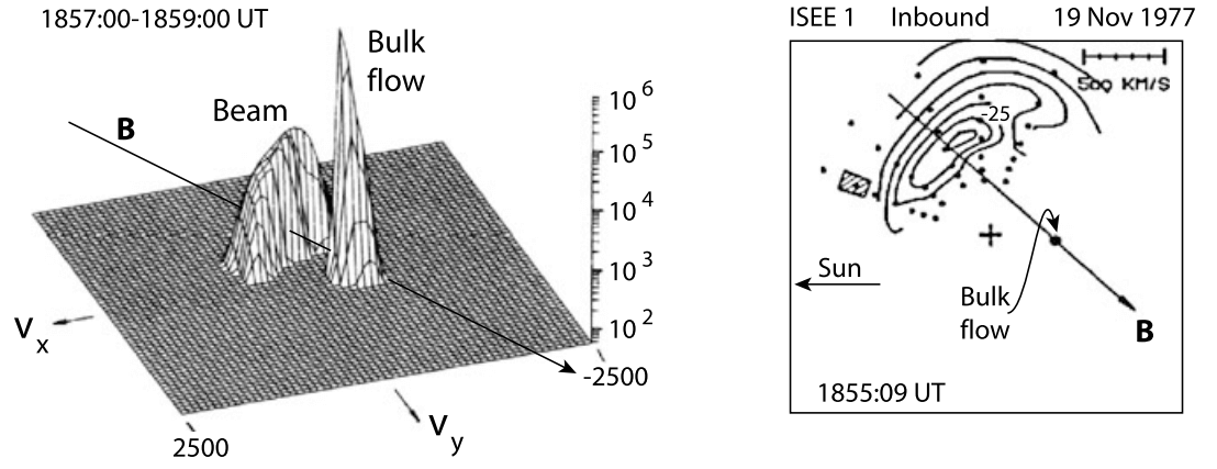
These beams along the foreshock boundary play some role in the foreshock dynamics as they seem to represent a source population for the entire ion foreshock. Whether and why this is really so is not yet fully understood as the shock should reflect ions at almost every place in its quasi-parallel state. However, it seems that only the group of ions that escape from the shock along the foreshock boundary can form such beams. This points on a further interesting relation between quasi-perpendicular and quasi-parallel shocks at a curved shock surface with a smooth transition from quasi-perpendicular to quasi-parallel as sketched in Figure 22.14 and realised in space, for instance, at planetary bow-shocks. It seems as so these beams escape from the quasi-perpendicular region of the shock along the nearly tangential field lines. This would also be in agreement with the observation [Gosling et al, 1984] that the foreshocks of extended interplanetary shocks do not show any signs of reflected ion beams. They are only very weakly curved being nearly planar, and do not possess a recognisable quasi-perpendicular area on the surface.
Kucharek et al. (2004) analysed ion distributions along magnetic field lines that were connected to the quasi-perpendicular area of Earth’s bow shock. Investigating the origin of those beams they found that, indeed, the observed ion beams at the foreshock boundary result from reflection at the quasi-perpendicular shock and that, without the presence of a quasi-perpendicular region, there would presumably be no distinct foreshock boundary and no ion beams escaping into the foreshock. If this is the case, then the population in the quasi-parallel ion foreshock is indeed provided by two different ion sources, the beams from the quasi-perpendicular shock region and the genuine foreshock ion population. The latter has no beam character but is rather a diffuse ion component [see also Meziane et al, 2004]. Interplanetary shocks possess only the latter one.
Roughly 2% of the ion inflow leaves the shock ramp upstream in the form of a beam along the magnetic field.12 Kucharek et al. (2004) argue that the ions which escape along the magnetic field, are reflected from the ramp/overshoot region where they have been in resonance with low-frequency plasma waves, which they assume to be large amplitude Alfvén-whistler waves. These ions experience pitch-angle scattering and pitch-angle diffusion towards small pitch angles, and subsequently can escape along the magnetic field in the upstream direction. Since the conditions for escape depend in the first place on the pitch-angle scattering process, the beams should be highly variable in time and location. The mechanism might still sound a bit speculative as long as no simulation proves its reality, but any mechanism which is able to pitch-angle scatter ions along the magnetic field in a quasi-perpendicular shock will naturally cause ion beams to escape from the ramp both in the upstream and in the downstream directions. Such simulations require a three-dimensional treatment which is not in reach yet.13
A measured example of the ion foreshock-boundary field-aligned ion beam distribution (Kis et al. 2004) is shown in Figure 21.18 for an upstream flow velocity \(V_1 \simeq 660\,\text{km}\,\text{s}^{-1}\), Mach number \(M_A = 8\), and average shock-normal angle \(\theta_{Bn} \simeq 15^\circ\), at an upstream distance from the Earth’s bow shock. This distribution is a so-called reduced distribution; it is the integrated over pitch-angle \(\phi\) and perpendicular velocity \(v_\perp\) magnetic field-aligned phase space distribution function \(f(v_\parallel) \sim 2\pi \int v_\perp^2 \mathrm{d}v_\perp f(v_\perp, v_\parallel)\) that has been appropriately binned and smoothed. The information to be taken out of this figure is that the reduced ion-beam distribution (solid line) is narrow in velocity, maximising at a speed (in absolute terms \(|V_{b\parallel}| \simeq 800\,\text{km/s}\)) that is only slightly larger than the parallel flow velocity (\(V_{1\parallel} \simeq 640\,\text{km/s}\), when taking into account the shock-normal angle), i.e. \(|V_{b\parallel}| \simeq 1.25V_{1\parallel}\). It is directed opposite to the flow. For comparison, a reduced parallel diffuse ion distribution is shown in the same plot taken deeper in the foreshock. This distribution is about symmetric to the magnetic field direction, indicating the about circular phase-space distribution of the diffuse ion component which appears as an energetic tail on the main ion distribution (note that the small gap on the left of the dashed diffuse-ion distribution curve is questionable as it dips below the 1-count level).
Meziane et al. (2004) reported CLUSTER observations of foreshock-boundary ion beams simultaneously with diffuse ions. They found that the nominal ion-beam velocity \(V_b \simeq 1.7V_1\) had no relation to any known shock-reflection mechanism like specular reflection, a conclusion which supports pitch-angle scattering as the beam-injection process as this is independent of the speed of the inflow.14
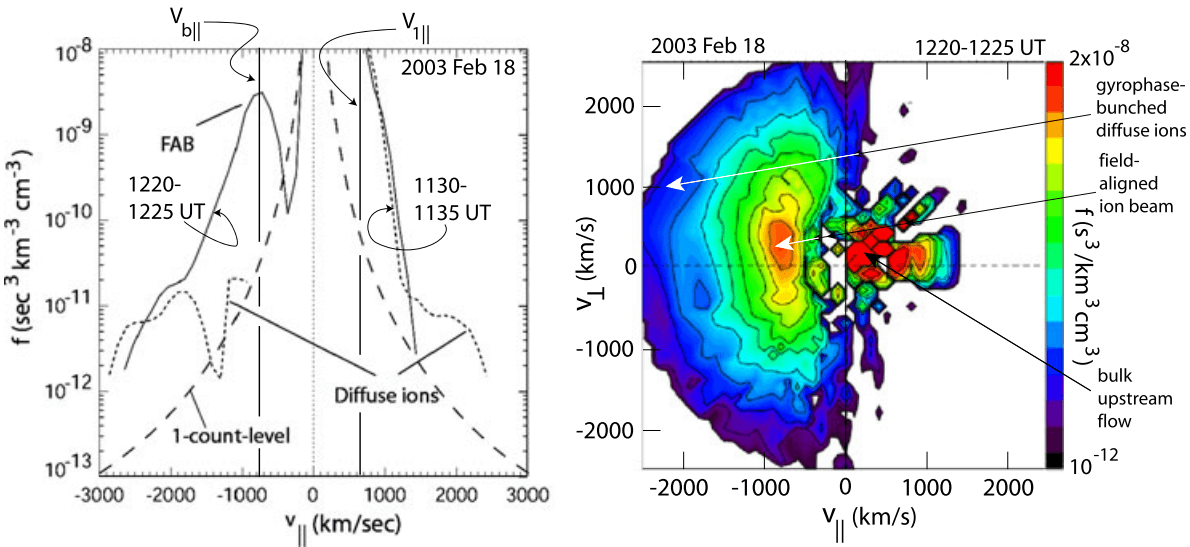
Kis et al. (2004) have carefully analysed the relation between the observed ion distribution at the upstream spacecraft position and the calculated shock-normal angle \(\theta_{Bn}\), determined from the local upstream magnetic field direction and the predicted shape of the bow shock. The result is shown in Figure 21.19 for three successive times on February 18, 2003 when the CLUSTER spacecraft was outside the bow shock. At 1130 UT and 1355 UT the shock normal angles \(\theta_{Bn} \sim 15^\circ\) and shock-spacecraft distances \(\sim 7.5\) respectively \(\sim 6.7\,\text{R}_\text{E}\) were similar. Despite this similarity the observed ion phase-space distributions were completely different. At 1130 UT no low-energy gyrating ions were observed, while they were present at the later time 1355 UT. Hence, at 1130 UT the spacecraft must have been closer to the ion foreshock boundary, i.e. the foreshock boundary was more inclined than at the later time such that beam particles scattered from the foreshock boundary have not arrived at the location of the spacecraft. Due to the velocity filter effect they have been separated out at spacecraft distance. The reconstruction of the position of the ion-foreshock boundary using the measured upstream conditions and shape of the shock for this period is shown in Figure 21.19. Indeed, at 1220 UT the spacecraft was close to the foreshock boundary and, as expected, detected the ion beam (as seen in Figure 21.18).
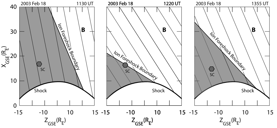
This observation supports the above advocated view that the ion-foreshock beam is generated in the transition region from quasi-perpendicular to quasi-parallel shock. The remaining questions to be answered are:
What pitch-angle scattering mechanism is responsible for the generation of such a beam?
What is the fate of the foreshock-boundary beam-ions during their propagation along the foreshock boundary?
Do they contribute to the foreshock ion population and if, in what way?
Currently we are not able to answer either of these questions definitely. In particular, the pitch-angle scattering mechanism is unknown or at least uncertain. When discussing wave generation, we will touch on the problem of the fate of the beam. Below we present evidence for the scattering of the beam ions and merging into the upstream foreshock diffuse-ion population.
21.5.2.2 Diffuse Ions
Reflected upstream magnetic field-aligned ion beams are observed at the foreshock boundary only. The second (and main) ion component encountered in the foreshock is the diffuse ion population which is detected there as the energetic extension of the inflow plasma. It is widely assumed that the origin of this component is also at the shock as there is no other energetic particle source available. However, close investigation of the diffuse ion component in the foreshock of the Earth’s bow shock wave has demonstrated that these ions are not produced in a specular reflection process at the shock. Rather their origin is of diffusive nature.
So far it has not been possible to identify the source of these ions though some models have been proposed which we will briefly discuss below in relation to the appearance of foreshock waves. These particles are also linked to the shock particle accelerations. Here, we merely discuss some of their properties and provide evidence that they are indeed coming from the shock, proving that the shock is an energetic ion source.
The foreshock-boundary ion beams also merge into the foreshock particle distribution by scattering from the foreshock boundary off their self-generated wave spectrum and subsequently being convected downstream by the bulk flow. Paschmann et al [1981] have mapped this merging process by following the evolution of the foreshock-boundary beam distribution shown in Figure 21.17 during the convection. In that figure the beam was detected close to the foreshock boundary. Figure 21.20 show its form deeper in the foreshock when it has spread substantially in angle evolving into half of a ring distribution already. Even deeper inside the foreshock the reflected ion distribution assumes the shape of a full ring around the bulk distribution as is shown in Figure 21.21.
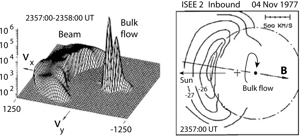
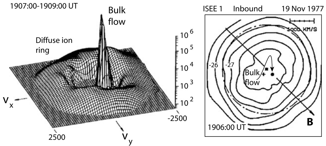
The evolution of the ion foreshock-boundary ion beam during its convection downstream into the foreshock and propagating deep inside the foreshock away from the ion foreshock boundary as has been seen by ISEE 2 and 1 on 04 November 1977. Velocities are in \(\text{km}\,\text{s}^{-1}\). The scale on the right is count rates, and background count rates were suppressed by choosing only values above \(50\,\text{s}^{-1}\). The direction of the magnetic field is also shown. The \(10^{-26}\) and \(10^{-27}\,\text{s}^3\,\text{cm}^{-6}\) level flux contours have been marked. [data from Paschmann et al, 1981]
The three observations depicted in Figures 6.4, 6.8 and 6.9 are from different times; it has, however, been checked that they are at distances corresponding to increasing distance from the foreshock boundary such that the assumption of the convectively processed beam evolution is well founded (or at least reasonable) even though it has not been directly proven.15 It is interesting to note that a gap remains between the original ion-phase space beam distribution and the bulk-flow distribution, which is another indication that the evolving distribution is part of the evolution of the ion-foreshock beam. Of a distribution that does not evolve out of a beam one expects a less regular behaviour and, generally, no such well expressed gap between bulk flow and beam in velocity space. In fact, the main energetic ion component in the foreshock is irregular and lacks a well expressd gap.
The discrepancy between the smooth no-gap foreshock distributions [Sentman et al, 1981a] and the gap-observations [Paschmann et al 1981] has, in fact, been noted much earlier [Sanderson et al, 1981; Scholer, 1985] without giving an explanation but suggesting a continuous ion source at the parallel shock. Below we provide further arguments for the two sources, foreshock-boundary beam and continuous extended shock-surface source hypothesis. Nonetheless, this conclusion must be taken with care because Figure 21.21 shows the gap progressively closing. Being sufficiently far, i.e. even farther away from the ion foreshock boundary then in this figure, it will not anymore be possible to distinguish between beam-evolved and genuine diffusive-ion distributions. Ultimately, both distributions will have merged indistinguishably. Still there is no agreement whether and where, i.e. at what distance from the ion foreshock boundary this merging of the two populations occurs.16
Trattner et al [1994], using AMPTE IRM measurements of diffuse ion densities upstream of the quasi-parallel bow shock found that the diffuse ion density decreases exponentially with shock distance. This investigation was substantially improved by Kis et al. (2004) in an attempt to infer about the source of the upstream diffuse energetic ions using the four CLUSTER spacecrafts. These authors determined the parallel-density gradient of diffuse ions in the energy range from 10 to 32 keV as a function of distance from the bow shock, as shown in Figure 21.22. We learned from this figure that in the deep foreshock, i.e. at distances far away from the ion-foreshock boundary, the diffuse ion component is densest close to the shock with density decaying exponentially with increasing upstream distance from the shock along the magnetic field. This spatial decay of the diffuse partial ion density \(N_i(\mathcal{E}, z) \sim \exp[-z / L(\mathcal{E})]\) is different for particles of different energy \(\mathcal{E}\). The e-folding distance \(L(\mathcal{E}) \sim \mathcal{E}\) turns out to increase linearly with energy, i.e. low energy particles are confined to the shock. The higher the ion energy the deeper can the ions penetrate into the upstream plasma. The proportionality constant determined from these data under the special conditions of the Earth’s bow shock is \(\sim 0.14 \text{R}_\text{E}/\text{keV}\). This behavior of the energetic foreshock ions provides indisputable evidence for the extended parallel shock-surface origin of the diffuse ion component. The source of the diffuse ions lies at the quasi-parallel shock. In order to be found at a distance upstream of the shock the ions undergo a diffusion process along the magnetic field. These ions are thus completely different from the beam ions found at the ion-foreshock boundary.
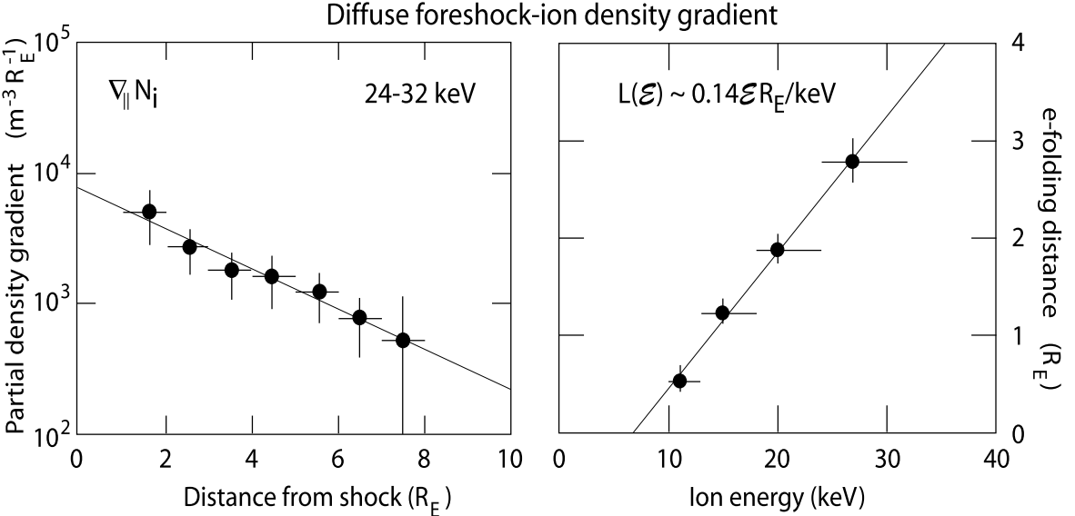
The e-folding distance for the diffuse ions is given by \(L(\mathcal{E}) = \kappa_\parallel(\mathcal{E})/V_1\), with spatial diffusion coefficient \(\kappa(\mathcal{E}) = \frac{1}{3}v l_\parallel(\mathcal{E})\), where \(l_\parallel\) is the diffusion length (parallel ion mean free path) and \(v\) the particle velocity17. From balance between convective inflow and diffusion into upstream direction, one can write \(l_\parallel(\mathcal{E}) = 3L(\mathcal{E})\sqrt{\mathcal{E}_1/\mathcal{E}} \sim \sqrt{\mathcal{E}/\mathcal{E}_1}\), where \(\mathcal{E}\) is the particle energy and \(\mathcal{E}_1\) is the upstream flow energy. In the solar wind the flow energy is a few keV, and a 20-keV diffuse ion will have a typical parallel diffusion length (or mean free path) of \(l_\parallel \sim (1−2)\text{R}_\text{E}\). This is a rather short distance, orders of magnitude shorter than the collisional mean free path of an ion. Hence, the diffusion estimate suggests that strong wave-particle interactions can be held responsible for the scattering and acceleration of the diffuse particle component, which enables it to diffuse and escape upstream from the shock and populate the foreshock. The diffusion process is energy dependent with the most energetic ions diffusing fastest.
These interactions should take place in the quasi-parallel shock transition because, as we have shown above, the diffuse upstream-ion density maximises closest to the shock. It is interesting to estimate the corresponding upstream-ion collision frequency \(\nu_\text{c,ui}\simeq \nu/l_\parallel\). For the 20 keV-upstream ions this yields \(\nu_\text{c,ui} \sim 0.2\text{Hz}\). This value is comparable to the ion cyclotron frequency \(\omega_\text{ci}/2\pi = (0.1−0.3)\,\text{Hz}\) in the \(B\simeq 8\,\text{nT}\) ramp magnetic field (Kis et al. 2004) during the time of observation.
It seems that waves, electromagnetic and/or electrostatic, related to the ion-cyclotron frequency are involved into the process of upstream ion diffusion. Since this diffusion is energy dependent, this process is not a simple pitch-angle diffusion as in the case of the generation of the ion beam that propagates along the foreshock boundary. The diffuse ion component must have experienced a substantial acceleration in this process, and this acceleration is located at or around the shock transition and contrasts with the ion-beam acceleration which is a scattering process followed up by pick-up acceleration when the upstream-propagating beam ions are subject to the effect of the main-bulk-stream convection-electric field in which they become accelerated in the direction perpendicular to the magnetic field to roughly four times the energy of the bulk flow, thereby evolving into the ring distribution that characterises their phase space distribution.
21.5.3 Low-Frequency Upstream Waves
In the frame of the upstream bulk flow the two ion components that populate the ion foreshock carry a substantial amount of free energy which is subject to dissipation. Since this dissipation is collisionless it can proceed only through the excitation of waves and wave turbulence through instability upstream of the quasi-parallel supercritical shock. On the other hand it is obvious that the presence of neither of the components can be understood without complete knowledge of the waves in the foreshock and their interaction with the particles.
Since their first detection by Olson et al [1969], Russell et al [1971], Fairfield [1974] and Fairfield & Feldman [1975], observation of shock-upstream waves has been a long-standing issue. Their existence was predicted by Tidman & Northrop [1968], followed by MHD [Barnes, 1970] and kinetic [Hasegawa, 1972] theories of electromagnetic wave excitation and propagation upstream of a collisionless quasi-parallel supercritical shock. Wu [1972] suggested that they might develop into discrete wave-packets as had been inferred from observation by Russell et al [1971]. The ISEE 1-3 spacecraft allowed for a more elaborate investigation of the properties of upstream waves. More recently, CLUSTER measurements have been used to investigate the temporal and spatial structure of upstream waves and wave turbulence. Wave generation is coupled to particle-energy loss and to particle scattering both playing a substantial role in particle acceleration. We start with a review of the properties of upstream waves in the ion-beam and diffuse ion region from observations and discuss mechanisms of their generation.
[Burgess 1997] reviewed the observed wave organizing by frequencies. He distinguished between Low Frequency Waves (5 mHz- few 100 Hz) and High Frequency Waves (>1 kHz), the latter covering the electrostatic waves from ion-sound to electron plasma waves, as well as radiation. Radiation generation will be discussed in detail later. Here, we only note the almost continuous presence of waves in the ion-acoustic band which have been known since Rodriguez & Gurnett [1975] to populate the complete foreshock region. These spectra might be composed of several different modes, ion-sound, electron-acoustic, Buneman modes, electron-cyclotron harmonics, and others. Their generation mechanism is not clear yet. They might, via a number of different instabilities, be the result of the presence of the hot foreshock-electron component, which also invades the ion foreshock, or they are excited by unresolved narrow electron beamlets that emanate from the quasi-parallel shock. They might also be excited by plasma inhomogeneities, spatial inhomogeneities in the electron distribution, or they are the result of nonlinear wave-wave interaction which is expected to take place in the foreshock. Little we have known about these high frequency waves since Burgess’ remarks.18
However, there has been substantial progress in the understanding of the low frequency waves and their role in quasi-parallel shock dynamics. The waves that are most important in shock formation propagate in the ultra-low frequency range <0.1 Hz. Usually they have large (magnetic) wave amplitudes, around \(|\mathbf{b}|/B \sim 0.2−1.0\), which identifies them as highly nonlinear. These large amplitude waves had already been observed by Russell et al [1971] to have wave forms from monochromatic to solitary waves, frequently with steep edges resembling shocklets and suggesting that the waves have experienced nonlinear steeping during their evolution and propagation. They sometimes show the typical signs of fluctuations that are connected to these edges and obviously propagate in the whistler mode. Thus these forms are indeed little shock-like structures.
In the same frequency window, large-amplitude pulsations have been identified. These are very typical for quasi-parallel shocks. Schwartz & Burgess [1991] and Schwartz et al [1992], identifying them in the AMPTE magnetic field measurements, coined the name SLAMS for them, which stands for Short, Large Amplitude Magnetic Structures. They are also known as upstream pulsations. Their duration is 10–20 s; they have very large amplitudes \(|\mathbf{b}|/B \sim 5\), indeed, but appear as a more coherent structure that is embedded in the ultra-low frequency wave turbulence. Like the ultra-low frequency waves, they propagate in upstream direction in the plasma rest frame while being swept toward the shock by the convective flow. Their polarization is mixed with – possibly – left-hand polarisation (in the plasma rest frame) slightly dominating, suggesting their ultra-low-frequency (ULF) wave origin. Sometimes the polarisation is different on both sides of the upstream pulsation, indicating that they have evolved by some process which produces both kinds of polarisation, which is similar to a solitary wave.
The propagation velocity of SLAMS exhibits an interesting amplitude dependence. The upstream directed pulsation speed increases with amplitude, which also is a solitary wave-like property. Moreover, they grow when approaching the shock and entering the increasing density gradient of diffuse ions, and they play an important role in shock reformation. Schwartz et al [1992] suspected that these pulsations are the building blocks of quasi-parallel shocks.
Another interesting property is that SLAMS contain thermal plasma with properties of the upstream flow, while being surrounded by the hot foreshock plasma. One would therefore believe that their source region is located at the ion-foreshock boundary. Being created there by an ion-ion beam plasma interaction they might grow nonlinearly until reaching quasi-equilibrium like solitary structures, having captured the upstream plasma, and afterwards being convected toward the shock into the heart of the ion foreshock.
21.5.3.1 Ion-Beam Waves
Each of the two different upstream-ion populations is responsible for the excitation of its own instabilities. In this section we deal only with those waves which are excited by the foreshock-boundary ion beam. Figure 21.18 suggests that the situation is that of an ion-ion beam interaction (for the moment neglecting the gyrophase-bunched diffuse-ion component). In the frame of the upstream flow the reflected foreshock-boundary ion beam propagates upstream along the magnetic field at parallel speed \(v_{b\parallel}\simeq -(2−3)V_{1\parallel}\), where \(V_{1\parallel}\simeq 600\,\text{km}\,\text{s}^{-1}\). The upstream ion temperature (in energy units) was \(T_i \simeq (1−2)\,\text{keV}\), yielding a thermal ion velocity of \(V_\text{i,th}\simeq 200\,\text{km}\,\text{s}^{-1}\). The beam can be taken as warm with thermal speed \(v_\text{b,th} \le v_{b\parallel}\). Hence, \(v_{b\parallel}> V_\text{i,th}\) with magnetized background and beam ions. On the other hand, the electrons are hot with \(T_e \simeq 100\,\text{eV}\).19
Expected Wave Modes Theoretically, we expect that the beam can excite long-wavelength negative-helicity Alfvén waves via the firehose instability when \(p_\parallel > p_\perp\). In addition, because the ion beam is mildly warm, it can excite the resonant left-hand ion-ion beam instability, which is possible for \(v_{b\parallel} > V_A\sim 100\,\text{km}\,\text{s}^{-1}\). When the beam thermal speed can be considered to be small, it may excite right-hand resonant ion-ion beam modes. Both modes propagate upstream along the magnetic field with the beam on the background of the upstream flow. They are not as fast as the beam, however, and are thus subject to downstream convection with the flow towards the shock. The firehose mode, at the contrary, moves against the beam and thus by itself moves downstream in the direction of the shock position when excited. A link to the plasma dispersion relations is discussed in Section 10.7.5.
In all three cases the foreshock-boundary beam will lead to the excitation of low-frequency Alfvén and ion cyclotron waves which in the shock frame approach the shock while having their source on the foreshock-boundary field line. During this shock-directed convection and/or propagation they populate the foreshock region with low frequency electromagnetic fluctuations, which might further interact with the diffuse foreshock-ion component. On the other hand, since the phase and group velocities \(\omega/k_\parallel\) \(\sim\) \((\partial\omega/\partial k_\parallel)\) \(\sim\) \(V_A\ll v_{b\parallel}\) of these waves are of the order of the Alfvén velocity and are, thus, much less than the beam and flow velocities, downstream convection will quickly remove them from the foreshock-boundary source region. Hence, their further evolution in the foreshock is determined by the competition between nonlinear wave steeping and – most important as will become clear below – interaction with the diffuse foreshock-ion component.
Including the electrons (while so far neglecting the electron foreshock component) leaves us with an ion-acoustic unstable phase-space configuration. In the upstream ion-plasma frame a relatively dense foreshock-boundary ion-beam is propagating upstream on a cold ion-hot electron plasma. In order to keep the plasma current-free the electron component is slightly retarded, creating conditions under which ion-acoustic waves can be excited. On the other hand, the configuration is not able to excite neither the Buneman-two stream instability the modified-two stream instability, because the beam propagates solely parallel to the magnetic field. This is shown in Figure 21.23. The instability is excited by the velocity difference between the ion foreshock-boundary ion beam \(F_\text{ib}(v_\parallel)\) and the slightly shifted to the left hot (\(T_e \sim 100\,\text{eV}\)) electron distribution because the velocity difference \(\Delta V\) between ion beam and electron component \(v_\text{e,th} > \Delta V\) \(\sim\) \(10^3\,\text{km}\,\text{s}^{-1}> c_\text{ia}\) \(\sim 100\,\text{km}\text{s}^{-1}\) exceeds the ion acoustic speed while being less than the electron thermal velocity \(v_\text{e,th}\). These ion acoustic waves occupy a relatively broad spectrum with downstream parallel phase velocities \(<v_\text{ib}\) and become swept towards the shock. Since they quickly leave the foreshock boundary and since the beam is not hot, ion-Landau damping in the source region plays no role. However, when entering the diffuse-ion foreshock region these waves encounter the hot diffuse ion component, will interact with it, and will thereby experience (positive and negative) Landau damping.
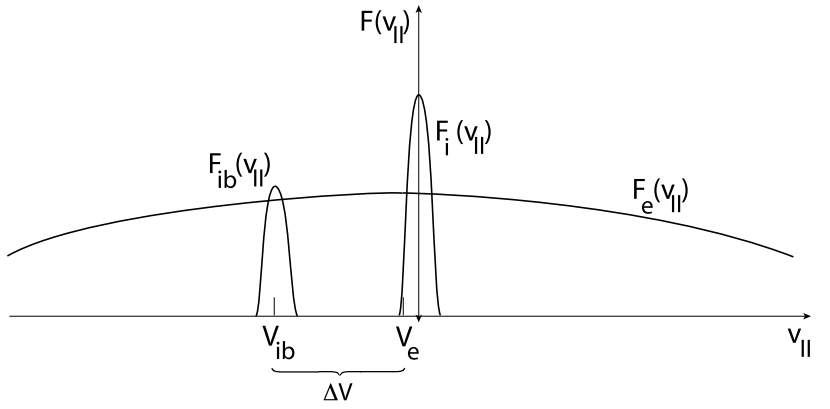
Observations Observationally, it is difficult to distinguish between foreshock-boundary waves and diffuse-ion generated waves. Two types of waves that can be related to the presence of the upstream beams have been reported in the vicinity of the bow shock. Fairfield [1974] and Fairfield & Feldman [1975] found monochromatic large-amplitude discrete wave packets in the frequency range \(\omega/2\pi ∼ 0.4\,\text{Hz}\) which Hoppe & Russell [1980] showed to be right-hand polarized whistlers at \(\omega \simeq 10\omega_\text{ci}\) propagating on the plasma rest frame and being unable to escape far upstream. The other class of waves is of smaller amplitude \(|b|/B \sim 0.1\) and frequency of the order of \(\omega/2\pi \sim 1\,\text{Hz}\). These waves form trains which are directly tied to the upstream foreshock-boundary ion beams [Hoppe et al, 1982]. In fact, as Hoppe et al [1982] demonstrated they occur only in the presence of the observed reflected 2−5 keV foreshock-boundary ion beams [Eastman et al, 1981] which Kis et al. (2007) have shown to evolve from a beam into a gyrating particle component that in the deep foreshock is superimposed on the diffuse ion component before it merges into it. However, as Feldman et al [1983] have shown from measuring the electron distribution function, it is not the ion beam who excites these whistlers. The probability that they are driven by the particular electron distribution in the foreshock is rather higher.
The waves observed propagated obliquely (\(<60^\circ\)) with respect to the magnetic field, at an average angle of \(\sim 45^\circ\). The observed spectrum and the dispersion relation determined from the measurements are shown in the high-frequency part of Figure 6.12. This figure has been combined from the high-frequency observations of Hoppe et al [1982] and the low-frequency observations of Le & Russell [1992], both obtained from the ISEE spacecraft measurements. Tentative wave numbers have been determined for the high-frequency waves from measuring the time delay of the wave front arrivals at the two spacecraft ISEE 1 and ISEE 2 spacecraft yielding (surprisingly) short wavelengths < 100 km. Knowing the wave number, the frequency has been back-Doppler shifted \(\omega=\omega_\text{ISEE} - \mathbf{k}\cdot\mathbf{V}_1\) into the plasma frame yielding unusually high frequencies \(\omega \sim (20−100)\omega_\text{ci}\). This procedure determines the dispersion relation (naturally with large errors as indicated by the bars), which is found to be about linear in the narrow high frequency range of the waves in the rest frame of the plasma. The waves that have been left-hand polarised in the spacecraft frame turn out to become right-hand polarised in the plasma rest frame.
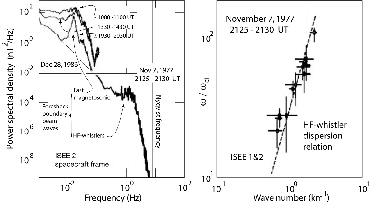
From these properties it was initially concluded that the waves propagate in the whistler branch and have been excited by the cool ion-ion beam instability, which would be consistent with our initial discussion. This conclusion is, however, questionable. The high rest-frame frequencies are not in agreement with model calculation [Sentman et al, 1981a; Gary, 1993] using the realistic observed beam properties. These yield wave frequencies of the order of \(\omega \sim 0.1\omega_\text{ci}\) for both the ion-ion beam and firehose modes. In fact, Eastwood et al. (2005) report CLUSTER observations of similar waves but with much lower frequency \(\omega/\omega_\text{ci} \sim 0.1\) and wavelength the order of \(\sim1\,\text{R}_\text{E} \sim 6000\,\text{km}\), which is in excellent agreement with the theoretical predictions. These waves are cold ion beam-excited fast-kinetic (magnetosonic) whistlers, in the terminology of Gary (1993) and Krauss-Varban et al [1994]. The high-frequency waves ∼1 Hz whistlers are instead most probably driven by the particular electron distribution in the foreshock [Feldman et al, 1983] rather than by the cold-ion beam instability. This claim is also supported by the fact that deeper in the ion foreshock, where the electron distribution becomes more isotropic, these waves do not occur separately from smaller magnetic field structures (SLAMS or shocklets).
In quite good agreement with the CLUSTER measurements are the ISEE foreshock waves analysed by Le & Russell [1992] who found the spectral peak at frequencies \(\omega \sim 10^{-2}\,\text{Hz}\) with the spectrum broadening with increasing distance from the ion-foreshock boundary. This is shown in the upper left part of the spectrum in Figure 21.24 where the measurements of Hoppe et al [1982] and Le & Russell [1992] have been combined. Even though the conditions on the two observation times were not identical, one finds that the high-frequency whistlers identified by Hoppe et al [1982] occur on the approximate high-frequency extension of the Le & Russell [1992] 1930–2030 UT spectrum which is closest to the ion foreshock boundary. Note, however, that the low-frequency part of the Hoppe et al [1982]-spectrum (not shown here other but indicated by a thin straight line in the figure) was flatter and in the (relatively short) overlap region with the Le & Russell [1992]-spectrum did not show any indication of the magnetosonic foreshock-boundary waves, which must be due to the particular conditions prevailing during this observation period. Thus the Hoppe et al [1982] waves are a (high frequency) wave species that is different from these more common low-frequency/long-wavelength fast-magnetosonic waves. These latter waves are also of much higher (∼5 orders of magnitude) spectral density as seen from Figure 21.24 and has been confirmed by the later CLUSTER measurements. Moreover, the magnetosonic waves are left-hand polarized in the plasma frame, and their compressive fast-magnetosonic character is proved from the in-phase variation of the density and magnetic field fluctuations shown in Figure 21.25.
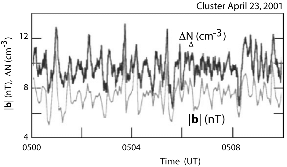
The presence of these low-frequency ion-beam generated waves implies that the ion beams interact with the fluctuating electromagnetic field. In this process they become scattered and diffuse in phase-space, which is the reason for the spreading of the ion beam in phase space and the final merging into the diffuse background distribution. Kis et al. (2007) have followed this evolution of the beam as we have described above. It is responsible also for the gradual spreading of the spectrum in the upper left part of Figure 21.24. A spectrum similar to that given there can be found in the paper of Kis et al. (2007). Archer et al [2005], from CLUSTER observations, inferred the nature of these ultra-low frequency (ULF) waves and showed that their correlation lengths along the wave vector direction k is of the order of 1−3\(\text{R}_\text{E}\), while it can be a factor of three larger in the direction perpendicular to \(\mathbf{k}\), rendering these waves oblate though nearly planar.
During times of hot beams Eastwood et al [2003] observed upstream propagating left-hand low-frequency waves which have been excited on the Alfvén-ion-cyclotron branch of the kinetic dispersion relation. These waves are kinetic Alfvén waves which have been excited by the hot upstream propagating beam similar to the one shown on the right in Figure 21.18. In the spacecraft frame these waves because they are swept downstream by the flow, appear as right-handed waves. Eastwood et al [2003] report that with onset of the waves the beam gets more diffuse. This can either be interpreted as the reaction of the waves on the beam or that the spacecraft enters the region where the initially cold beam enters the foreshock, spreads in velocity and after becoming hot enough generates the observed waves.
Simulation studies available of the evolution of the reflected ion beam and the generation of upstream waves is still of great interest as of 2024!
21.5.3.2 Diffuse Ion Waves
Long-period ∼30 s waves are the rule in the foreshock. They occur together with the diffuse foreshock-ion component [cf., e.g., Sanderson et al, 1983; Mellott, 1986] which is located deeper inside the foreshock. Because of this reason, any waves that are excited by the diffuse ion component are restricted to the interior of the foreshock. One even has defined some fuzzy boundary of these waves called ULF-wave boundary [Russell & Hoppe, 1983; Greenstadt & Baum, 1986], which is even more inclined against the upstream magnetic field than the ion-foreshock boundary and outside of which the ULF wave activity should be weak. The reason is that ULF waves, if propagating upstream, can move at most with fast-magnetosonic velocity which for a supercritical shock is smaller than the stream and also less than the reflected ion beam velocities. The advection by the flow will blow them downstream towards the shock and confine them to a region relatively close to the shock bounded to upstream by the ULF-boundary.
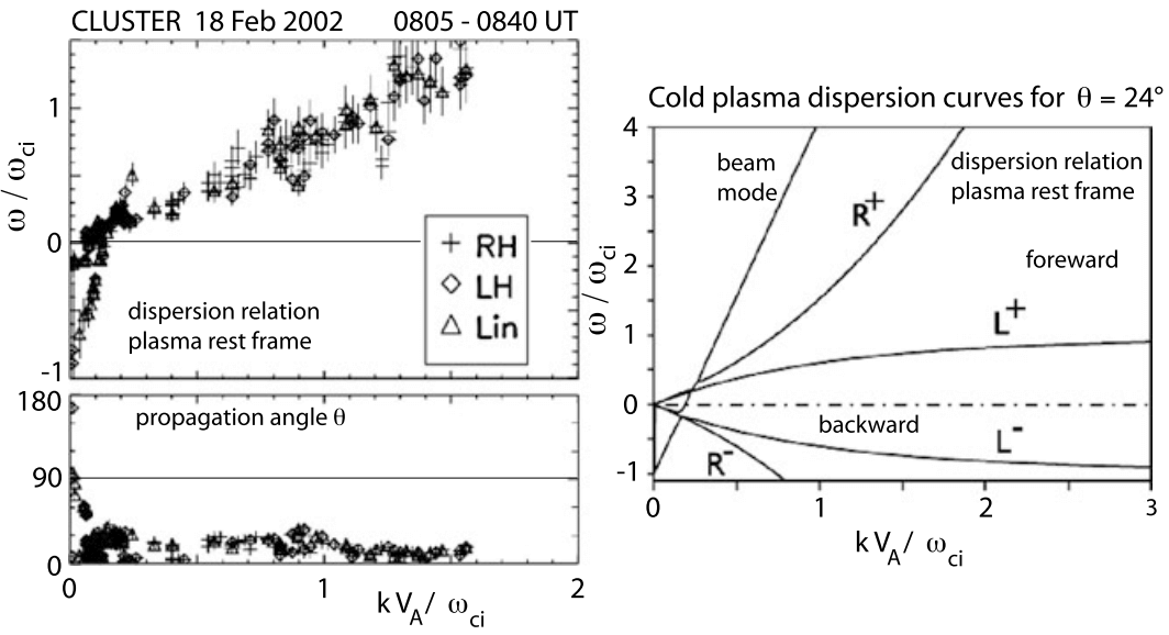
The dispersion relation of the low-frequency waves in the foreshock from the three-dimensional observations of CLUSTER is given in Figure 21.26. The left part of the figure shows the dispersion relation in the plasma rest frame and the angle of wave propagation with respect to the local average upstream magnetic field. The scatter is quite large. Nevertheless it is surprising to find a well expressed nearly linear part on the dispersion relation even though the dispersion relation is composed of the contributions of several distinct modes with different polarizations. The representation is linear, which, on the k-axis, emphasises the short wavelengths (larger k values). From linear theory one expects that the long wavelengths (small k) should be more pronounced. Unfortunately, this region could not be resolved sufficiently at the available CLUSTER separation distances at that time. These low frequency waves, in the plasma frame, seem to propagate close to perpendicular to the magnetic field and, therefore, are probably in the fast magnetosonic mode. Moreover, it seems that a straight beam dispersion relation contributes to the perpendicular propagating waves. It also seems that in the low-frequency (magnetosonic) waves have negative frequency (i.e. propagating in opposite direction). Linear dispersion theory for the parameters during the observation time yields the curves on the right in the figure showing the coupling between the presumable beam mode and the four plasma modes at wave numbers \(kV_A/\omega_\text{ci} < 0.3\). The experimentally determined dispersion relation resembles this clustering of couplings at small k and very low frequencies ω. However, application of linear theory is dangerous if not questionable because the foreshock plasma is highly disturbed, the low frequency waves have rather large amplitudes and can barely be considered as linear waves. In addition the plasma is highly inhomogeneous exhibiting steep gradients in density and magnetic field. For an Alfvén speed \(V_A \simeq 30\,\text{km}\,\text{s}^{-1}\) and an ion-cyclotron frequency \(\omega/2\pi \simeq 1\,\text{Hz}\), wavelengths around the linear wave coupling are of the order of \(k/2\pi \simeq 100\,\text{km}\) and should thus be affected by the plasma inhomogeneities (note that decreasing the reference cyclotron frequency decreases the wavelength even further). Nevertheless, at the very low frequencies and very long waves the waves are probably in the fast magnetosonic wave band.
More mysterious are the higher frequency-short wavelength waves. From comparison with the linear dispersion relation they seem to fit on the right-handed whistler branch (high frequency magnetosonic whistler \(R^+\)). However, inspection of the dispersion relation indicates that all kinds of polarization are scattered along the dispersion curve. The curve itself is very irregular even though the propagation angle of the waves seems to be about constant at weakly oblique angles. This wave composition suggests that we are not dealing here with one single wave mode but rather with the short wavelength part of a turbulent spectrum which has generated all kinds of short wavelength fluctuations with different almost randomly distributed polarization in a forward cascading process from long to short wavelengths. This idea has been elaborated in more detail in Narita et al [2006] who found that the shorter wavelength spectrum is indeed about featureless and power-law, close to a \(-5/3\) -Kolmogorov-spectrum of stationary turbulence with most of the power in the perpendicular (non-compressive) magnetic component providing another argument for Alfvénic and magnetosonic turbulence. This is shown on the left in Figure 21.27. The figure also indicates the respective gyro- and inertial wave numbers, \(k_\text{ci} = v_i/\omega_\text{ci}\) and \(k_\text{in} = c/\omega_\text{pi}\). There is indication that the spectra change slope at around these numbers due to onset of anomalous ion viscosity and ion inertia. The large maximum on the perpendicular power curve near \(k \sim 10^{-3}\,\text{km}^{-1}\) corresponds to a wavelength of \(\lambda \sim 6000\,\text{km}\) reported earlier [e.g., Eastwood et al, 2003] and is at the right position for energy injection by low frequency instability.
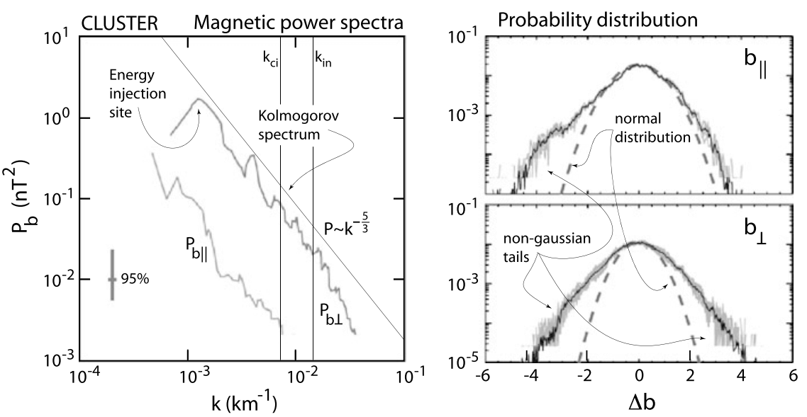
However, the conclusion that the deep foreshock is subject to fully developed fast magnetosonic/Alfvénic turbulence is by no means fully justified. This becomes obvious from considering the probability distribution of the field fluctuations as given on the right in Figure 21.27. Would the fluctuations be normally distributed then their distribution functions would have the shape of the dashed curves. Instead the distributions are skewed into tails. In the case of the parallel component the distribution lacks symmetry. Such tails may indicate that the turbulence is non-stationary, intermittent or inhomogeneous. All three cases might hold in the foreshock, in particular as the foreshock is a rather limited spatial region which is bounded from two sides and is subject to plasma injections and plasma losses. Nevertheless, the spectra determined contain signs of strongly nonlinear and turbulent interactions, and the waves, particularly the low-frequency waves, are of large amplitude and interact with the plasma ion component as also with other waves. These waves affect the upstream backstreaming ion component scattering, heating and accelerating it. On the other hand the upstream ion component is responsible for the existence of the waves as it is the ultimate energy source of the waves. And, to close the cycle, the waves cannot escape upstream very far from the foreshock since in a supercritical shock the Mach number of the flow is higher than any Mach number based on the wave speed and is thus high enough for the flow to advect the wave spectrum towards the shock. As long as the waves do not completely dissipate their energy during this convection, the electromagnetic wave energy accumulates at the location where they arrive at the shock.
The consequence of this accumulation is that the waves affect the shock, cause instability of the shock surface, and reorganise the shock front. This makes quasi-parallel shocks principally non-stationary (or as sometimes said, turbulent) and subject to some kind of irregular reformation. One may thus expect that a supercritical quasi-parallel shock does not represent a solid shock surface over a large area. It consists of a more or less dense “patchwork” of areas which together form a shock but which also appear and disappear in an irregular manner, come and go, and organise the shock in a certain volume where the entropy increases but where a multitude of very difficult to handle processes take place that can be investigated only experimentally or with the help of properly designed numerical simulations.
An important question that has not been addressed anywhere in the investigation of the ion-foreshock dynamics concerns the role of the foreshock electron component which, in the large ion-foreshock domain, consists of two populations, the ∼100 eV upstream electron population which belongs to the quasi-neutral upstream flow, and the hot ∼ several kev-electron population which is the product of the shock reflected electrons we are going to discuss in the next section. This component is isotropic but irregular and might contribute to ion-foreshock instabilities thereby affecting the foreshock turbulence and shock formation.
21.5.4 Electron Foreshock
Even though the ion-foreshock occupies the larger part of the foreshock and, which is more important, plays the decisive role in the dynamics of a quasi-parallel supercritical shock, it would be an ignorant attitude not to mention the part that aside of the main flow is populated solely by the reflected higher energy electron component, i.e. the electron-foreshock region. Schematically its extent and relation to the ion-foreshock is shown in Figure 22.14. The electron foreshock has been identified already by Scarf et al [1971] in the OGO 5 satellite observations. Scarf et al [1971] noted the occurrence of enhanced electron fluxes near the bow shock, which were related to observations of high-frequency electric-field spikes at 30 kHz. They concluded that these spikes resulted from Langmuir waves that had been excited by electron beams arriving from the bow shock along shock-connected magnetic field lines.20 It could be confirmed that these electron fluxes were magnetic-field aligned and of higher energy than the bulk electrons in the main flow. This was interpreted as electron beams emitted into upstream direction from the shock, even though no mechanism was known that could provide the required shock-electron acceleration/reflection – in fact, a de Hoffman-Teller-frame shock-reflection mechanism had already been proposed by Sonnerup [1969] and was reinvented and elaborated on for electrons much later by Wu [1984].
21.5.4.1 Electron Beams
In analogy to the ion-foreshock boundary the electron-foreshock boundary (which is the ultimate upstream boundary of the foreshock) carries narrow bursts of electron beams, which escape into upstream direction from the shock along the magnetic field and which are slightly displaced by the convective flow into downstream direction.
An example of a narrow energy spectrum of such a beam measured by the IMP-8 satellite is shown on the left in Figure 21.28. The spacecraft was in the electron foreshock boundary for a relatively short time only. Being near apogee, the spacecraft was about standing. Thus the short contact time with the beam most probably indicates that the electron-foreshock boundary is fairly narrow or that the electron beams are bunched into electron bursts. The electron beam also occupies only a small volume in velocity space corresponding to a narrow bump on the distribution [Anderson et al, 1981]. Only one energetic electron-gyroradius deeper in the electron foreshock the electron beam becomes depleted and just forms an energetic tail of hot halo electrons on the electron distribution function of the flow.
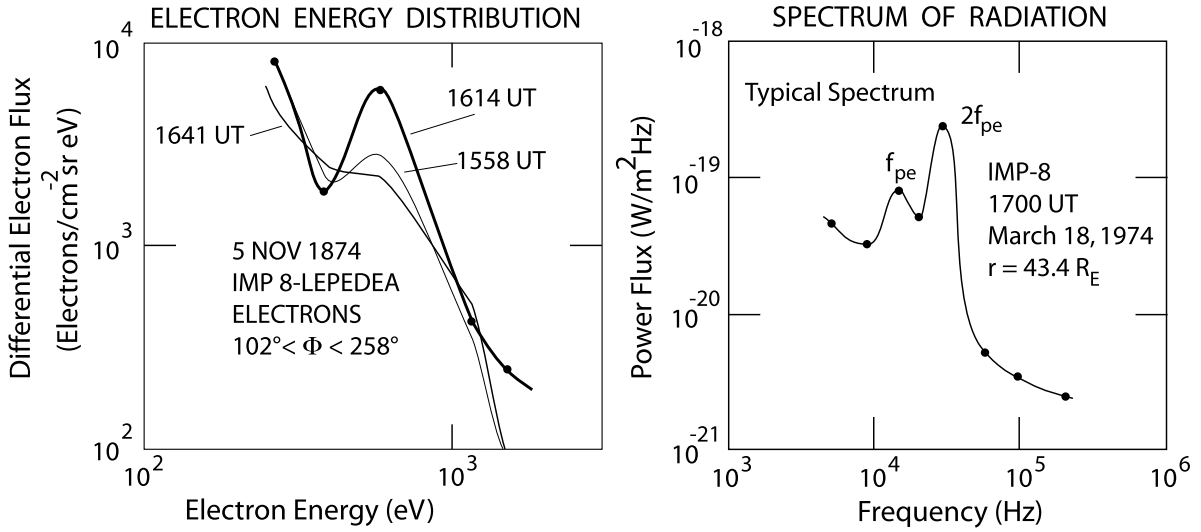
Figure 21.29 shows electron phase-space observations from the electron instruments on ISEE 1 & 2 during crossings of the electron-foreshock boundary. The left part of the figure [taken from Fitzenreiter et al, 1984] is a much higher time and velocity (respectively energy) resolution plot than that in the former figure. It is nicely seen how the electron distribution evolved from a field-aligned (nearly) Maxwellian distribution prior to contact with the foreshock boundary, through a field-aligned-beam-like distribution at contact, into a distribution with an energetic tail along the magnetic field, where the electron beam has been completely washed out. This transition takes place within a time interval of 15 s, just allowing to obtain the three measurements. The pseudo-three-dimensional plot of the electron distribution function on the right was obtained on another day when the spacecraft passed the electron-foreshock boundary and a series of distributions were recorded from upstream, across the foreshock boundary, and into the electron foreshock. Here only the foreshock-boundary distribution is shown when the narrow electron beam has evolved flowing into upstream anti-shockward direction along the magnetic field. Note the narrow angular extension of the beam, its weakness, and its comparably large velocity which allows to identify it just outside the bulk of the hot ∼100 eV background electrons which are much hotter than the beam (indicated by the small beam width in \(v_\parallel\)).
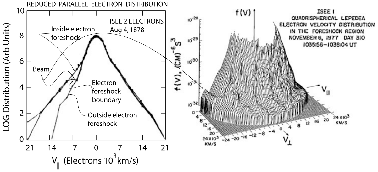
The conclusion that can be drawn from these observations, which in the follow-up time had also been confirmed by measurements of other spacecraft like AMPTE IRM and AMPTE UKS, is that, similar to the ion foreshock, the electron foreshock consists of a very narrow region along about the shock-tangential upstream-magnetic field line (or flux tube) which is populated by a cold, weak, and fast electron beam, and a broad electron region adjacent downstream of this flux tube where the electron distribution exhibits tails and in addition contains a hot, fairly isotropic electron component. The electron beam (like the ion beam at the ion-foreshock boundary) has its origin near the shock-tangential magnetic field line which is connected to the quasi-perpendicular part of the shock. The mechanism of its generation has not yet been unambiguously clarified. Presumably it consists of a combination of the de Hoffman-Teller frame mechanism of Sonnerup [1969] and the bending of the shock surface plus some kind of stochastic acceleration in the electric fields which evolve in the shock transition, ramp and overshoot. Such fields have indeed been reported recently on scales below the electron skin depth \(d_e = c/\omega_\text{pe}\) to be very large, of the order of \(\le 100\,\text{mV}\,\text{m}^{-1}\) parallel and perpendicular to the magnetic field [Bale & Mozer, 2007]. The presence of the hot electron component in the foreshock, on the other hand, is not due to this reflection mechanism but requires another mechanism that heats and accelerates electrons at a quasi-parallel shock over a large area of its surface.
Langmuir Waves
So-called ‘gentle electron beams’, which are just those beams one observes at the electron-foreshock boundary – fast, but not too fast (\(V_b\) few times \(V_1\)), parallel (\(V_b \equiv V_b, V_{b\perp} = 0\)), weak (\(N_b \ll N_e\)), cool (\(v_{eb} < v_e \ll V_b\)), are know to be the drivers of Langmuir waves with dispersion relation \[ \omega^2(\mathbf{k}) = \omega_\text{pe}^2 + 3 v_e^2 k^2,\quad v_\text{res} > \sqrt{3}v_e \] via the resonant kinetic gentle-electron beam instability. The Langmuir resonance conditions is \(ω − \mathbf{k}\cdot\mathbf{v}_\text{res} = 0\), where \(\mathbf{v}_\text{res} \sim \mathbf{v}_b\) is the resonant electron velocity. Combining it with the dispersion relation, it is easy to see that in order for the wave number k to be real the resonant velocity must satisfy the condition on the right in the above equation.
Electron Foreshock-Boundary waves
Figure 21.30, taken from Décréau et al [2001], shows a beautiful double passage of the CLUSTER-spacecraft quartet through the Earth’s bow shock on December 22, 2000 in the light of the CLUSTER plasma wave spectrum recorded by the WHISPER plasma wave instrument aboard the four CLUSTER spacecraft. Figure 21.31 shows an example of these high-resolution measurements.
CLUSTER came from the magnetosphere, entered the downstream region of the shock, passed the shock to upstream, re-entered the shock, and escaped downstream again. The relevant signatures of each region are seen in all four spacecraft. The uppermost light blue trace is the electron plasma frequency \(f_\text{pe} = \omega_\text{pe}/2\pi\) which maps the local plasma density. The shock appears as the intense broadband emission with maximum intensity in the low-frequency waves. In the density it is mapped as a steep drop in \(f_\text{pe}\) to the low upstream density values. Close to the shock a number of intensifications in \(f_\text{pe}\) can be recognised. These occur at the time of contact with the electron foreshock boundary when intense plasma waves are excited in the Langmuir mode. It is interesting to note that the intensifications occur in spots and are not necessarily narrow-band. They may exceed \(f_\text{pe}\), or they may also drop below it: the plasma frequency may have ‘hair’ or ‘beards’. Moreover, sometimes intense lower-frequency emissions are detected half way between the plasma frequency and the low frequency emissions in the foreshock. The most intense of these emissions belong to the region closer to the shock where the density gradient has not yet settled to the upstream values, but weaker emissions of the same kind occur farther away in the upstream low density domain.
It is highly suggestive that the observed intense spots in the plasma frequency, with the ‘hair’ parts exceeding and the ‘beard’ parts hanging down from the local fpe, are related to magnetic field-aligned electron beams emanating from the shock and propagating upstream along the electron foreshock-boundary magnetic field as these are the same signatures as those observed with the ISEE and AMPTE spacecraft, though with much better frequency resolution and higher sensitivity here. Taking into account that the upstream plasma frequency away from the shock is fairly constant this implies that the shock-normal angle \(\theta_{Bn}\) changes on an irregular and fast time scale, i.e. that the direction of the upstream magnetic field is highly variable even under conditions of apparent quiescence in the upstream medium. The conclusion drawn from this would not be that the upstream magnetic field is subject to violent variations as in the electron foreshock there is no reason for the magnetic field to be strongly affected. Rather this variability points on the temporal variation of the shock area near the tangential field line. Even a small change in the shock normal there will cause a large variation in the location of the tangential magnetic flux tube at a distance upstream of the shock. The main reason is that the super-critical shock is neither in thermal nor in thermodynamic equilibrium and is thus by its very nature subject to changes in all its physical parameters.
21.5.4.2 Radiation
Shocks are frequently referred to as sources of radiation. Famous examples are supernova shocks, which are visible in almost all wavelengths, from radio through visible light up to x-rays [e.g., Dickel & Wang, 2004], and solar type II shocks with their main radiation signatures seen in the radio waves.
Supernova shocks are relativistic shocks which are not treated here. Their Mach numbers range from weakly relativistic to highly relativistic, but the energy per particle in them remains to be less than the rest energy of an electron, \(m_e c^2 = 0.511\,\text{MeV}\), which allows to treat them classically. This does not hold anymore for the central supernova engine which drives the flow and which in some cases results in the generation of ultra-relativistic jets. There the shocks become non-classical, and not only radiation losses but also particle generation must be taken into account in their description.
Theory of shock-emitted radiation is based on plasma processes which under the prevailing collisionless conditions in the shock and foreshock plasmas refer to wave-wave coupling as the main generation mechanism. Direct emission from particles is unimportant, because the energy losses a particle experiences when becoming retarded or reflected at a shock, are not transformed into radiation. In all non-relativistic cases radiation losses can completely be neglected compared with all other energy losses. Nevertheless, the observed radiation is of interest because in many cases, where no measurements are possible to be performed in situ, radiation is the only direct and presumably identifiable signature a shock leaves, when seen from remote. The other signature is the generation of energetic particles, which will be treated next, but energetic particles are a more diffuse indicator of a shock, because their propagation is vulnerable to scattering from other particles, obstacles and, in the first place, scattering by magnetic fields.
21.5.5 Quasi-Parallel Shock Reformation
In quasi-parallel supercritical shocks there is not such a stringent distinction between the region upstream of the shock and the shock itself like in quasi-perpendicular shocks. The foreshock and the shock itself cannot be considered separately due to the presence of the reflected and diffuse particle components in the foreshock. These are the source of a large number of waves.
The interaction of these waves with the shock is one of the main issues in quasi-parallel shock physics. In the present section this will become clear when we will be dealing with the formation, behaviour and structure of quasi-parallel shocks as it has been inferred less from observation than from numerical simulations. The reason is that the real observations in space do not allow to separate the particles and waves from the shock. They all occur simultaneously and are interrelated and can never be observed in their initial state. The observations to which we will nevertheless occasionally refer will leave the impression of large-amplitude noisy fluctuations.
21.5.5.1 Low-Mach Number Quasi-parallel Shocks
It is usually assumed that low-Mach number shocks are stable, i.e. show no substantial time variation or reformation. It is not completely transparent why this should generally be so.
- The critical Mach number has been shown by Kennel et al [1985] to become small at narrow shock normal angles \(\theta_{Bn}\to 0\), in which case even low-Mach number quasi-parallel shocks should become supercritical and reflect ions.
- Any fast ions of parallel velocity \(v_\parallel > V_1\) that have been heated in the shock can in principle escape from the quasi-parallel shock upstream along the magnetic field and should appear in the foreshock where they contribute to wave generation.
Therefore, it makes sense to investigate the state of quasi-parallel shocks in view of their stability and wave generation even for low Mach numbers. In addition, any waves that are generated in the shock ramp or transition with upstream directed \(\mathbf{k}\) and fast enough parallel phase or group velocities could also escape from the shock in upstream direction. This could, in particular, be possible just for low Mach number quasi-parallel shocks.
To check this possibility Omidi et al [1990] have performed one-dimensional hybrid simulations finding that initially the quasi-parallel shock consisted of phase-standing dispersive (magnetosonic) whistler waves with the last whistler wave cycle constituting the shock ramp. As expected, the wave vectors of these phase-locked magnetosonic whistlers are aligned with the shock normal. At later times, backstreaming ions along the upstream magnetic field excite a long-wavelength whistler wave packet upstream of the shock. In the one-dimensional simulation the wave vector is restricted to the shock normal while it is known from theory that the growth rate is largest along the magnetic field. These oblique whistler waves should thus show up in two-dimensional simulation and may be visible at larger distance for sufficiently large upstream phase velocities.
Such two-dimensional (hybrid) simulations with a non-inertial electron fluid have been performed by Scholer & Fujimoto [1993] for a Mach number of MA = 2.2 and angles \(\theta_{Bn} = 20^\circ, 30^\circ, 45^\circ\) and by Dubouloz & Scholer [1995] for an angle \(\theta_{Bn} = 30^\circ\) and high Mach number MA = 5 (Figure 21.32). The lower Mach number simulations show the presence of a substantial number of backstreaming ions which cause an ion-ion instability in the upstream region. However, the excitation and properties of the waves depend strongly on the shock normal angle. Initially, as in the case of Omidi et al [1990] phase-locked short-wavelength whistlers appear which are replaced at later times by upstream long-wavelength whistlers with phase velocity directed and amplitude growing towards the shock ramp but upstream directed group velocity, i.e. the shock radiates energy away towards upstream, as one would naively expect, because the shock being supercritical must reject the excess inflow of energy which it can do by both, reflecting particles and emitting waves into upstream direction. These waves are excited by the backstreaming ion component in a strongly nonlinear interaction process because of the evolving steep ion-density gradient, which is of the same scale as the whistler wavelength. The \(\mathbf{k}\)-vector turns away from the magnetic field having comparable components parallel to \(\mathbf{B}\) and parallel to the shock normal \(\hat{n}\). For small \(\theta_{Bn}\) a remnant of the initial phase-locked whistlers survives but disappears at \(\theta_{Bn} = 30^\circ\). Close to the shock, where the backstreaming ion density is high, the waves have short wavelengths, and \(\mathbf{k}\) is almost parallel to \(\hat{n}\). In the high Mach number simulations no shock is produced but instead reflected ions were artificially injected with same Mach number as the incoming flow but with much higher temperature \(v_i = 14.1V_A\), forming a spatially uniform ion beam. The intention was to investigate the effect of the hot reflected ions. This is shown on the right in the above figure. The result resembles the former one where a shock was generated by reflection at a wall, but the effect in the injected beam case is stronger because of the higher Mach number. Hence it is the hot reflected ion component that is responsible for the wave dynamics and the shock dynamics.21
All this can be seen from the two-dimensional intensity contours of these waves in the foreshock, which are plotted at a relatively early time in the shock evolution in the simulations in Figure 6.26. On the right in this figure the geometry is given, with the magnetic field fluctuation vector \(\mathbf{b}\) in the (y,z)-plane. The bottom panel on the left shows contours of the \(b_z\) fluctuations in the (x,z)-plane. The nominal shock ramp is at \(x \approx 145 d_i\) at this time. The upper panel shows the non-coplanar component \(b_y\)-contours in the same representation. Behind the shock the fluctuations are irregular and disorganised. However, in front of the shock a clear wave structure is visible with strongly inclined wave fronts and of roughly \(\sim 10 d_i\) wavelengths in z parallel to the nominal shock surface. The wavelength in x is about three times as short.
These waves are seen in both components, \(b_z\), \(b_y\), are low amplitude at large distance from the shock but reach very large amplitudes simultaneously in both components during shock approach while, at the same time, bending and assuming structure in z-direction that is different from the regular elongated shape at large distance. This deformation of wave front may be due to the residual whistlers near to the shock, but it implies that the shock has structure on the surface in both directions x and z and is not anymore as planar as was initially assumed. The shock becomes locally curved on the scale of the shock-tangential wavelength. The waves deform the shock and, in addition, being themselves of same amplitude as the shock ramp, become increasingly indistinguishable from the shock itself. The shock is, so to say, the last of the large-amplitude magnetic wave pulsations in downstream direction, and the shock-magnetic field is not anymore coplanar, because the waves have contributed a substantial component by that points in the direction out of the coplanarity plane.
We have emphasised this phrase, because it expresses the importance of the low-frequency upstream magnetic waves in quasi-parallel shock physics. Contrary to quasi-perpendicular shocks where the reflected gyrating ions in combination with the reflected-ion excited modified-two stream instability were responsible for the shock dynamics and different kinds and phases of shock reformation, quasi-parallel shock reformation and much of its physics is predominantly due to the presence of large-amplitude and spatially distinct upstream waves. These are the generators of the shock and, due to their presence, the shock changes its character. It is highly variable in time and position along the shock surface and is – close to the shock transition on a smaller scale – ‘less quasi-parallel’ (or more perpendicular, i.e. the shock-normal angle \(\theta_{Bn}\) has increased on the scale of the upstream waves). The latter is due to the out-of coplanarity-plane component of the upstream waves. This conclusion remains basically valid also in full particle simulations. It had been suggested already earlier on the basis of ISEE 1 & 2 observation of the evolution of the upstream ultra-low frequency wave component [Greenstadt et al, 1993].
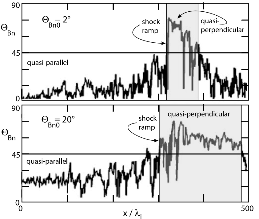
The gradual evolution of the shock normal angle ΘBn has been demonstrated in other hybrid simulations by Scholer & Fujimoto [1993] and Dubouloz & Scholer [1995] who investigated the evolution of the shock normal angle in dependence on distance from the shock. This is shown in Figure 21.33 for two-dimensional hybrid simulations with initial shock-normal angles \(\theta_{Bn0} = 2^\circ\) and \(\theta_{Bn0} = 20^\circ\), respectively, which we anticipate here. In both cases ΘBn evolves from quasi-parallel to quasi-perpendicular angles. Qualitatively there is little difference between the two cases. At the shock ramp \(\theta_{Bn}\) is deep in the domain of quasi-perpendicular shocks. The only difference is that for the nearly parallel case the angle jumps to quasi-perpendicular quite suddenly, just before approaching the shock ramp, while the evolution is more gradual for the larger initial \(\theta_{Bn}\). In both cases the evolution is not smooth, however, which is due to the presence of large-amplitude foreshock waves. Transition to quasi-perpendicular occurs for the initially nearly parallel case at the nominal shock ramp while for the initially quasi-parallel case it occurs at an upstream distance of about \(100 d_i\) from the shock. This is sufficiently far away for the upstream flow ions to feel the change in the shock normal.
One notices that this transition is on the ion scale, implying that in the region close to the shock the ions experience the shock occasionally (because of the large fluctuations in \(\theta_{Bn}\)) – and when ultimately arriving at the shock – as quasi-perpendicular. It is thus not clear, whether the electrons do also see a quasi-perpendicular shock, here (which cannot be concluded from these hybrid simulations, however). The ISEE measurements of the electron distribution function by Feldman et al [1983] at the shock do not show a difference between quasi-perpendicular and quasi-parallel shocks. This fact suggests, in addition that, close to the shock transition, quasi-parallel shocks behave like quasi-perpendicular shocks as well on the electron scale, which is just what we have claimed.
We finally note that the behaviour of the shock normal angle gives a rather clear identification of the location of the shock transition in the quasi-parallel case, as indicated in Figure 21.33 by shading. Three distinctions can be noticed:
At larger initial shock-normal angles the transition to quasi-perpendicular angles occurs earlier, i.e. farther upstream than for nearly parallel shocks. This is due to the stronger effect of the large amplitude upstream waves in this case;
At larger initial shock normal angles the quasi-perpendicular shock transition is considerably broader than for nearly parallel shocks, i.e. it extends farther downstream before the main quasi-parallel direction of the magnetic field in the downstream region takes over again and dominates the direction of the magnetic field
At an initial shock-normal angle of \(20^\circ\), this region is \(\sim 150d_i\) wide, implying that the magnetic field direction behind a quasi-parallel shock remains to be quasi-perpendicular over quite a long downstream distance measured from the shock ramp. For the nearly parallel shock this volume is only about \(\sim 50d_i\) wide.
This observation must have interesting implications for the physics downstream of quasi-parallel shocks. For instance, applied to the Earth’s bow shock, where \(d_i \sim 10^3\,\text{km}\). both distances correspond to regions wider than the order of \(> 5\text{R}_\text{E}\) which is larger than the nominal width of the magnetosheath! Thus, behind the bow shock a substantial part of the magnetosheath plasma should behave as if the bow shock would have been a completely quasi-perpendicular shock.
21.5.5.2 Turbulenct Reformation
When speaking about turbulent reformation we have in mind that a quasi-parallel super-critical shock is basically a transition from one lower entropy plasma state to another higher entropy plasma state that is mediated by a substantially broad wave spectrum. Such a transition has been proposed by Schwartz and Burgess (1991) based on the detection of the large amplitude magnetic pulsations (SLAMS) in the foreshock.
Figure 21.34 on the left shows this model assuming that somewhere upstream in the foreshock magnetic pulsations have been excited which become convected downstream toward the shock by the convective flow, grow in amplitude and number and accumulate at the shock transition to give rise to a spatially and temporarily highly variable transition from upstream of the shock to downstream of the shock. An important clue in this argument was the observation that, first, the pulsations grow in amplitude when approaching the shock and that, second, they slow down. This slowing down is effectively an increase in their upstream directed velocity on the plasma frame with growing amplitude such that their speed nearly compensates for the downstream convection of the flow.
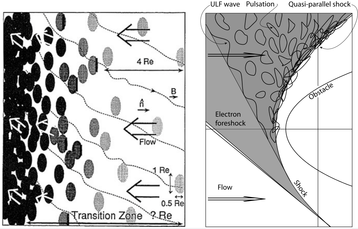
On the right of the figure, which is suggested by the observations of Kis et al. (2007), a larger region is seen. Here the pulsations are the result of growing ULF waves which are generated in a volume inside the foreshock but relatively close to the ion-foreshock boundary. These waves grow to large amplitudes until evolving into pulsations which the flow carries toward the shock. Growth, slowing down, and accumulation then lead to the pile up of the pulsations at the shock location and formation of the turbulent shock structure. Only the shock-tangential upstream magnetic field lines are plotted in the right figure. In the left part, several field lines are schematically shown exhibiting the fluctuations imposed by the background level of ULF fluctuations. Moreover, a certain bending of the field lines is included here in approaching the shock transition with the field lines turning more perpendicular the closer they come to the shock. This bending is what we claim to be a parallel shock turning quasi-perpendicular at a scale very close to the shock. In this schematic drawing, however, there would be no reason for the magnetic field to turn this way. What closer observations and simulations show is that the turning of the field is the result of the presence of the large amplitude magnetic pulsations. This will become clearer below.
Observations
Of course, the model shown in Figure 21.34 is a schematic model only which, however, has some merits in explaining the observations. The signature of a quasi-parallel shock in the magnetic field is indeed quite different from that of a quasi-perpendicular shock. The magnetic signature of a quasi-parallel shock is quite broadband in that it lacks a clear location of the shock front, which contains a broad region of very large amplitude compressive oscillations in magnetic magnitude and in the direction of the magnetic field that subsequently is recognized as a passage across the quasi-parallel shock.
An example is shown in Figure 21.35 as measured by the CLUSTER spacecraft. This figure shows eight hours of observation by CLUSTER in the immediate vicinity of the quasi-parallel shock. It is difficult to say where in the figure the shock transition is located as the large fluctuations in the magnetic field magnitude and directions mask the various back and forth passages across the shock that are contained in the data. Clearly, at the beginning near 1400 UT the spacecraft was in the downstream region. The fluctuations show that during almost the entire sequence the magnetic field exhibits compressive fluctuations. These belong to the shock transition. At the same time large fluctuations in the direction of the magnetic field are also observed. In the compressions of the magnetic field buried are also upstream pulsations (SLAMS), and many of the changes in direction belong to the ULF waves present at and near the shock. The changes in direction indicate that the shock does not behave like a stationary flat surface. Instead, it shows structure with highly fluctuating local shock normal directions.
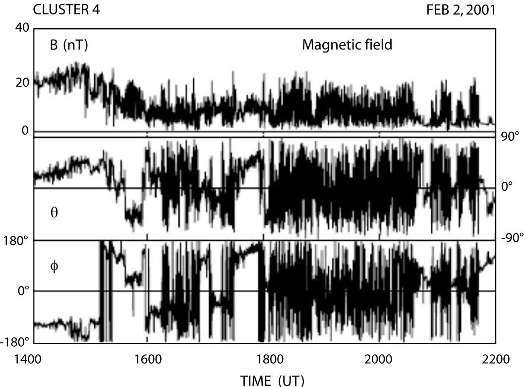
Lucek et al. (2002) checked this expectation by determining the local shock-normal angle \(\theta_{Bn}\) and comparing it with the prediction estimated from magnetic field measurements by the ACE spacecraft which was located farther out in the upstream flow. The interesting result is that during the checked time-interval of passage of the quasi-parallel shock the prediction for the shock normal was around \(20-30^\circ\), as expected for quasi-parallel shocks. However, this value just set a lower bound on the actually measured shock normal angle. The measured \(\theta_{Bn}\) was highly fluctuating around much larger values and, in addition, showed a tendency to be close to \(90^\circ\). It strengthens the claim that quasi-parallel shocks are locally, on the small scale, very close to perpendicular shocks, a property that they borrow from the large magnetic waves by which they are surrounded. In fact, we may even claim that locally, on the small scale (\(\sim\mathcal{O}(d_i)\)), quasi-parallel shocks are quasi-perpendicular.
The data suggest that, indeed, the quasi-parallel shock is the result of a build-up from upstream waves which continuously reorganise and reform the shock. Figure 21.36 shows three representative examples of such upstream waves which are far from being continuous wave trains. The upper panel is taken from the large density fluctuation region in the shock transition. This region turns out to consist of many embedded magnetic pulsations (SLAMS) of very large amplitudes. In the present case amplitudes reach \(|\mathbf{b}| \sim 25\,\text{nT}\). These pulsations have steep flanks and quite irregular shape, exhibit higher frequency oscillations probably propagating in the whistler mode while sitting on the feet or shoulders of the pulsations. It is most interesting that the different CLUSTER spacecraft – at spacecraft separation <1000 km – do not observe one coherent picture of a particular pulsation. This implies that the pulsations in the shock are of shorter scale than spacecraft separation: the different spacecraft observe different structures respectively different pulsations. In addition, the magnetic field directions (not shown in the figure) are very different from spacecraft to spacecraft and thus from pulsation to pulsation, and even for one pulsation at its front edge and trailing edge different magnetic field directions are observed. The directions of the magnetic normal across a pulsation change on very short spatial scales. The quasi-parallel shock front has thus a rather irregular shape, which will be bent locally with changing direction of its normal.
The second panel shows an isolated pulsation farther away from the shock transition. This pulsation exhibits a much more coherent way on the four different CLUSTER spacecraft. It seems as if the pulsation is still in evolution as three of the spacecraft see a nearly coherent structure while the fourth which is farther away sees it in a different state. Concluding from this event, isolated pulsations seem to have larger dimensions and lower amplitudes, which would be consistent with the assumed solitary properties of pulsations. The third panel shows a shocklet, i.e. a structure which presumably has little in common with pulsations. It is embedded into long wavelength ULF wave trains, evolves into steep front and drives whistlers attached to this front across the flow. These waves were already observed by Russell et al [1971]. Their properties indeed resemble those of sub-critical little shocks which propagate against the flow, though with slower speed such that they effectively are slowly convected towards the shock. Observations of plasma wave spectra by AMPTE IRM are shown in Figure 6.31. There the large amplitude SLAMS pulsations appear as broadband wave signatures resembling narrow shock structures.
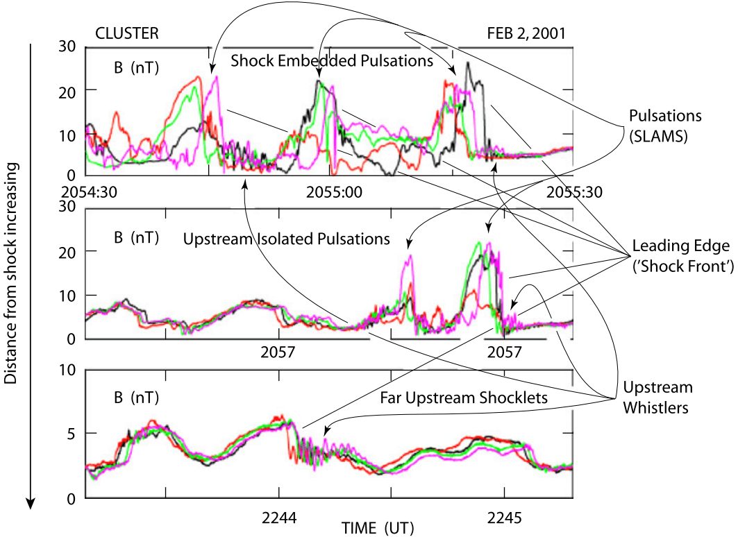
Another interesting property of magnetic pulsations in the shock transition region where they overlap to form the quasi-parallel shock is presented by Behlke et al [2003]. Measurement of the electric cross-SLAMS potential identify a substantial unipolar drop in the electric potential of several 100 V, corresponding to a potential ramp, when passing from upstream to downstream across the pulsation. Such a drop signifies the presence of an electric field in one direction across the pulsation. Taking the mean size of a pulsation to be roughly 1000 km, the mean electric field is \(\left<E\right> \simeq 400\text{mV}\,\text{m}^{-1}\). However, this field drops mainly at the leading edge of the pulsation. Such a field presumably corresponds to a steep pressure gradient in the pulsation.22
The measurements of Behlke et al [2003] anticipated the later report of strong electric fields in the shock by Bale & Mozer [2007]. In addition to this observation it was found [Behlke et al, 2004] that the single pulsations were subject to a fairly large number of high frequency/Debye scale structures in the electric field seen in the WHISPER recordings (bottom panel), which belong to electron holes or solitons which form in the pulsation gradient regions as shown in Figure 6.32. The bipolar electric field and unipolar potential across one – indeed very symmetric – soliton is seen in this figure. These observations suggest that the pulsations are indeed the main constituents of a quasi-parallel shock with the dynamics on the micro-scale of a quasi-parallel shock going on mainly in the single pulsations of which the shock transition is built.
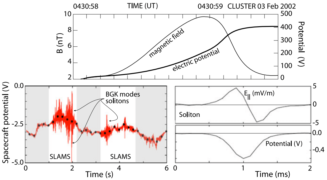
The occurrence of these intense nonlinear electrostatic electron plasma waves at the quasi-parallel shock transition is intriguing. It forces one to draw another very important main conclusion from these observations: that quasi-parallel shocks are sources of electron acceleration into electron beams, which are capable to move upstream along the magnetic field over a certain distance and excite electron plasma waves at intensity high enough to enter into the nonlinear regime, forming solitons and electron holes (BGK modes). This is possible only if quasi-parallel shocks are quasi-perpendicular as well on the electron scale.
Indeed, electron reflection into beams which generate Langmuir waves is presumably possible only when in the supercritical quasi-parallel shock transition region the magnetic field changes from quasi-parallel to quasi-perpendicular on the electron scale \(\sim d_e\). Indications of such a change on the ion scale \(d_i\) have been noted above at a number of occasions, but the detection of solitary structures in the electron plasma waves in relation to quasi-parallel shock transitions provides a very strong argument for this to be true on a scale which is well below the ion scale. Only if this is the case, there will be ample reason for electrons to become reflected and accelerated into beams from the transition region in a quasi-parallel shock. As we already noted, we may, therefore, expect that quasi-parallel supercritical shocks on the electron scale are not anymore quasi-parallel but change to become locally quasi-perpendicular, while on the larger ion scale they still remain quasi-parallel. Because of this reason high Mach number quasi-parallel shocks will be embedded into a diffuse high energy electron component that emits radiation.
If this conclusion will turn out to be true, it will have important consequences for collisionless shock physics. Supercritical, collisionless, nonrelativistic shocks will, in fact on the electron scale, always behave quasi-perpendicularly, and it may be suspected that this conjecture will also hold for relativistic shocks though probably for other reasons (like the generation of transverse magnetic fields by the Weibel instability, which becomes dominant in relativistic shocks [see, e.g., Jaroschek et al, 2004, 2005]). This implies also that the true quasi-parallel shock physics cannot be properly elucidated when ignoring electron effects as is, for instance, done in hybrid simulations.
1D Hybrid Simulations
We do already know from the observations that quasi-parallel shocks exist at small \(\theta_{Bn}\) with their foreshocks being populated by a diffuse ion component that excites upstream waves and mediates the beam-generated upstream ion-foreshock boundary waves. The impossibility for this diffuse component of being entirely due to shock reflection in the quasi-perpendicular part of the shock, immediately proves that the quasi-parallel (or even the nearly parallel shock) must be able to reflect particles upstream. Hence, either a quasi-parallel shock is capable of generating a large cross-shock potential, or it is capable of stochastically – or nearly stochastically – scattering ions in the shock transition region in pitch angle and energy in such a way that part of the incoming ion distribution can escape upstream, or – on a scale that affects the ion motion – a quasi-parallel shock close to the shock transition becomes sufficiently quasi-perpendicular that ions are reflected in the same way as if they encountered a quasi-perpendicular shock.
Observations suggest that the latter is the case, while observations also suggest that large potential drops occur in the large-amplitude magnetic pulsations (SLAMS) where they accumulate in the shock ramp [Behlke et al, 2004]. Hence, reflection of ions will be due to the combination of both effects, the electric potential drop and the magnetic deflection. In fact, this can be a quite complicated process for an ion passing across a number of magnetic pulsations, in each of which it is being retarded and at the same time deflected by a small angle until its normal velocity component is decreased sufficiently that a further deflection in pitch angle suffices to let it return into the upstream region.
Early hybrid 1D simulations have already confirmed some characteristics of quasi-parallel shocks. First 1D hybrid simulations in an extended simulation box [Burgess, 1989] suggested that the reformation of quasi-parallel shocks is about cyclic and is caused by the impact of large-amplitude upstream waves. Scholer & Terasawa [1990], using \(\theta_{Bn} = 20^\circ\) and MA = 3.5 with an upstream ion thermal velocity \(v_{th,i} = V_A\)$ (corresponding to \(\beta_i = 1\)) in 1D hybrid simulations (with small numerical resistivity) showed that the reflected ions are not coming from the core of the incident upstream ion distribution but originate in the shell of this distribution, having initial velocities \(v \simeq 1.7v_{th,i}\). These ions escape from the shock quite far upstream and excite ULF waves with upstream directed velocity of \(\sim 1.3 V_A\) at distances up to \(> 300 d_i\), which are convected downstream to reach the shock. In this 1D hybrid simulation the only mode in which they can propagate is the compressive fast magnetosonic mode.
These waves are in fact what in observations has been identified as pulsations (SLAMS) but is not yet recognized as such, here. During downstream convection the waves grow and slow down in the interaction with the foreshock ion component. When approaching the shock they generate a large amount of new reflected ions. These slow the incident ion population down and steepen the wave crest, which becomes the new shock front. In the time between the arrival of the compressive waves the shock is about stationary and develops phase-locked upstream whistlers which the arriving next wave crest destroys. From these simulations it could not be concluded what process produced the reflected ions, however, as 1D simulations among suffering from other eficiencies select only one particular direction of wave numbers and are thus not general enough for drawing final conclusions.
The nature, generation and effects of the large-amplitude upstream waves have been further investigated in more detail in 1D [Krauss-Varban & Omidi, 1991; Scholer & Burgess, 1992; Scholer, 1993, among others], and in 2D hybrid simulations [Krauss-Varban & Omidi, 1993; Scholer, 1993; Dubouloz & Scholer, 1995]. Since shocks are three-dimensional, it is clear that two-dimensional numerical simulations at same resolution come closer to reality. However, they suffer from restrictions in size of the simulation box and simulation time. Since reality does not confront us with an initial state, large boxes and long times are needed.
In order to identify a particular wave mode, the dispersion of the wave must be investigated. This dispersion relation depends on the frame in which it is taken, because the energy/frequency of a wave is not invariant with respect to coordinate transformations; in a medium moving with velocity \(\mathbf{V}\) it is Doppler shifted according to \(\omega^\prime = \omega(\mathbf{k}) - \mathbf{k}\cdot\mathbf{V}\), where \(\omega(\mathbf{k})\) is the dispersion relation in the rest frame of the flow. While the Doppler shift at high frequency is negligible, it completely changes the dispersion of ultra-low frequency waves at large Mach numbers. Figure 21.38 on its left shows the deformation of the fast mode dispersion relation in the shock frame at large Mach number M > 1 and for waves propagating upstream in the plasma frame. The deformation causes negative frequencies of the waves which imply downstream directed phase velocities, which is nothing else but the intuitive downstream convection of the waves by the flow. However, the minimum in the dispersion relation implies that waves of a particular frequency and wave number have zero group velocities. In the shock frame the energy of these waves is stationary. Smaller wave numbers have energy moving downstream, larger wave number have energy moving upstream away from the shock. The right part of the figure shows simulations of upstream waves according to 1D hybrid simulations by Krauss-Varban & Omidi [1991] for \(\theta_{Bn} = 30^\circ\) and a Mach number \(M_\text{A} = 2.8\). The entire dispersion of the simulated waves is negative. The waves are all convected toward the shock as their Mach number is less than the streaming Mach number. Near the shock most of the wave energy moves downstream and will cross the shock. Still some shorter wavelength waves (large k) move in energy upstream in the shock frame. Farther away from the shock most of the wave energy encountered is seen to move upstream.
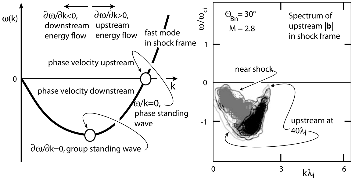
Scholer [1993] investigated these waves further in one-dimensional hybrid simulations performing several numerical experiments on them, taking away the shock and instead injecting a diffuse ion component from downstream. The main finding is that the large amplitude upstream magnetic pulsations (SLAMS) evolve out of the ULF wave spectrum in the interaction with the diffuse ion component. In accord with observation the pulsations move upstream in the plasma frame. Thereby their upstream leading edge steepens and is right-hand circularly polarised like required for whistlers. However, dispersion is unimportant: the main cause of the evolution of large pulsations is nonlinearity when the wave interacts with the diffuse ion distribution. This distribution has a steeper shock directed density gradient than the pulsation wavelength. Moreover, the flow becomes decelerated at the leading edge of the pulsation (as is seen in Figure 21.32), and here the velocity difference between the flow and the diffuse ion component drastically decreases, which shifts the k vector of the resonant wave to larger values, and the wavelength decreases during convection of the pulsation toward the shock.23 The standing whistlers in the leading edge are simply generated by the current flowing in the edge. It is thus concluded that it is the gradient in the hot diffuse ion component over a length of the same order as the wavelength which produces the pulsations. Ultimately these pulsations cause a quasi-periodic reformation of the shock, as we have described earlier, which thus has been proven by 1D hybrid simulations. The same result is obtained when the simulation starts right away without a shock but with an injected hot beam (which is no surprise as the generation of the shock, before it was removed in the former simulations in order to keep with the wave field, was due to the plasma flow-reflected ion beam interaction).
2D Hybrid Simulations
The 2D evolution of the pulsation (SLAMS) was studied later by Scholer & Fujimoto [1993] and Dubouloz & Scholer [1995] (see Figure 21.32). It basically confirmed the conclusions drawn from 1D simulations with the following three important modifications:
- The wave fronts of the pulsations (SLAMS) rotate into a direction that is more parallel to the shock thereby increasing the shock-normal angle locally to become quasi-perpendicular.
- The pulsations have short wavelength in shock normal direction, but are of substantially longer but finite lengths in the direction tangential to the shock, which provides structure to the shock in tangential direction.
- Shock reformation is a result due to the steeping and accumulation of the pulsations and is a quasi-periodic process, but the downstream structure of the shock over some distance is caused by the downstream convection of the old shock front, i.e. the bulk of the pulsations that had accumulated at the location of the former shock transition.
It is interesting to note that from one reformation cycle to the next rather large fluctuations in the magnetic field and density exist in the transition from upstream to downstream which are capable of trapping particles. The 2D simulations do also confirm the conclusion that the diffuse upstream ion component is responsible for the growth of the pulsations (SLAMS). The 2D simulations by Dubouloz & Scholer [1995], in particular, followed the same scheme as the 1D simulations, injecting hot diffuse ions into upstream in order to control the interaction between the diffuse ion component and large amplitude pulsations (SLAMS).
Full Particle PIC Simulations
In hybrid simulations, the ions are macro-particles while the electrons represent a charge-neutralising background. Clearly, such simulations are unrealistic if whistlers become involved.
21.5.6 Parallel Shock Particle Reflection
There are two possible mechanisms:
- A quasi-parallel shock is capable of generating a large cross-shock potential, or it is capable of stochastically – or nearly stochastically – scattering ions in the shock transition region in pitch angle and energy in such a way that part of the incoming ion distribution can escape upstream.
- On a scale that affects the ion motion, a quasi-parallel shock close to the shock transition becomes sufficiently quasi-perpendicular that ions are reflected in the same way as if they encountered a quasi-perpendicular shock.
21.6 Instabilities and Waves
In the context of collisionless shocks the instabilities of interest can be divided into two classes. The first class contains those waves which can grow themselves to become a shock. It is clear that these waves will be of low frequency and comparably large scale because otherwise they would not evolve into a large macroscopic shock. The primary candidates are magnetosonic, Alfvén and whistler modes. A number of waves can form secondarily after an initial seed shock ramp and grow in some way out of one of these wave modes: these are ion modes which have now been identified to be responsible for structuring, shaping and reforming the shock. In fact real oblique shocks — which are the main class of shocks in interplanetary space and probably in all space and astrophysical objects — cannot survive without the presence of these ion waves which can therefore be considered the wave modes that really produce shocks in a process of taking and giving between shock and waves.
The second class includes waves that accompany the shock and provide anomalous transport coefficients like anomalous collision frequencies, friction coefficients, heat conductivity and viscosity. These waves are also important for the shock as they contribute to entropy generation and dissipation. However, they are not primary in the sense that they are not shock-forming waves.
Among them there is another group that only carries away energy and information from the shock. These are high-frequency waves, mostly electrostatic in nature, produced by electrons or when electromagnetic they are in the free-space radiation modes. In the latter case they carry the information from remote objects as radiation in various modes, radio or x-ray to Earth, informing of the existence of a shock. In interplanetary space it is only radio waves which fall into this group as the radiation measure of the heliospheric shocks is too small to map them into x-rays.
Here we restrict mostly to low frequency EM waves in warm plasma, \(\omega\le \omega_{ci}\), while only mention the high frequency EM waves in the end. Such waves are excited by plasma streams or kinetic anisotropies in one or the other way. A simple summary is given in Table 21.3.
| Mode | Wave Type | Handedness | Other Properties |
|---|---|---|---|
| Firehose | Alfvén | left | Parallel prefered anisotropy |
| Ion-Ion Beam | Fast | right | Cool beam |
| Ion cyclotron | Alfvén | left | Warm beam |
| KAW | Alfvén | right | Electron, parallel electric field |
| Whistler | Alfvén | right | Hall term, electron |
21.6.1 Ion Instabilities \(\omega \leq \omega_{ci}\)
21.6.1.1 Firehose mode
The simplest instability known which distorts the magnetic field by exciting Alfvén waves that propagate along the magnetic field is the firehose mode. The wave excited are ordinary Alfvén waves, however, and are not suited for shock formation.
When the ion beam is fast and cold it does not go into resonance because its velocity is too high. In this case all ions participate in a nonresonant instability which in fact is a thermal firehose mode where the ion beam has sufficient energy to shake the field line. This mode propagates antiparallel to the ion beam, has small phase speed and negative helicity. This mode has large growth rate for large \(n_b / n_e\) and \(v_b / v_A\) simply because then there are many beam ions and the centrifugal force is large while the beam velocity lies outside any resonant wave speed. This instability becomes stronger when the ion beam is composed of heavier ions as the larger mass of these increases the centrifugal force effect.
21.6.1.2 Kinetic Alfvén waves
KAWs (Section 10.8.4) possess a finite \(E_\parallel\) which can accelerate electrons; in the other way, electron moving along the magnetic field in the opposite direction become retarded and feed their energy into KAWs.
Normally this is likely to be a minor effect, as the interaction of ions which are reflected from a solitary pulse and move back upstream ahead of the pulse will cause a stronger instability. The reflected ions will represent a beam that is moving against the initial plasma inflow which by itself is another ion beam neutralised by the comoving electrons. The free energy presented in the two counter-streaming beams leads to various instabilities as viewed by Gary (1993).
21.6.1.3 Kinetic growth rate
At low frequencies it suffices for our purposes of understanding shock physics to deal with a three-component plasma consisting of two ion species and one neutralising electron component which we assume to follow a Maxwellian velocity distribution. Moreover, we assume that the drifting ion components are Maxwellians as well. In conformity with the above remarks on a resonant instability we assume that the dominant ion component has large density \(n_i\gg n_b\), and the second component represents a weak fast beam of density \(n_b\) propagating on the ion-electron background with velocity \(v_b \gg v_i \approx = 0\). Following Gary (1993) it is convenient to distinguish the three regimes:
- cool beams (\(0<v<v_b\))
- warm beams (\(v\sim v_b\))
- hot beams (\(v\gg v_b\))
Figure 21.39 shows the beam configurations for these three cases and the location of the wave resonances respectively the position of the unstable frequencies.
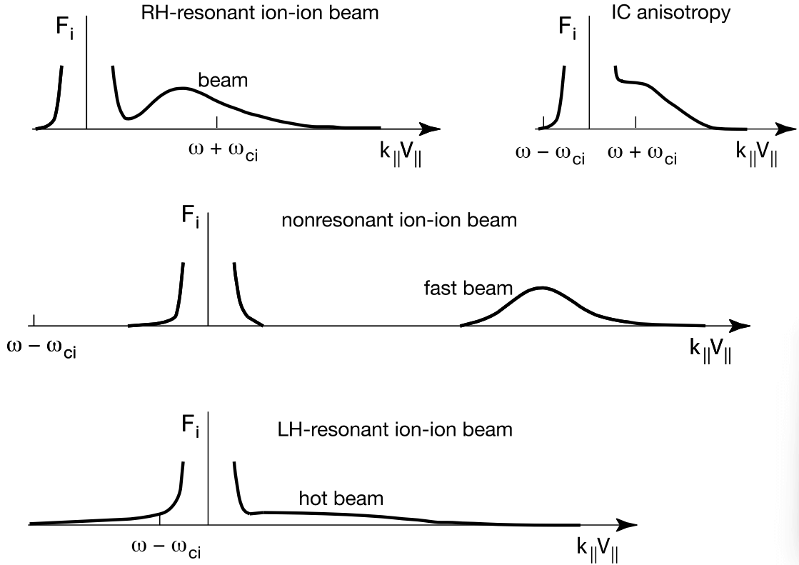
21.6.1.4 Cold Ion Beam: Right-Hand Instability
Assume that the ion beam is thermally isotropic and cool, i.e. its velocity relative to the bulk plasma is faster than its thermal speed. In this case a right-handed resonant instability occurs. In the absence of a beam \(v_b=0\) the parallel mode is a right-circularly polarised magnetosonic wave propagating on the lowest frequency whistler dispersion branch with \(\omega\approx k_\parallel v_A\). In presence of a drift this wave becomes unstable, and the fastest growing frequency is at frequency \(\omega \simeq k_\parallel v_b - \omega_{ci}.\) This mode propagates parallel to the beam, because \(\omega>0\), \(k_\parallel > 0\), and \(v_b > 0\). The numerical solution of this instability for densities \(0.01 \le n_b/n_i \le 0.1\) at the wave-number \(k_\parallel\) of fastest growth rate identifies a growth rate of the order of the wave frequency \(\gamma\sim\omega\) and \[ \gamma_m \simeq \omega_{ci}\left( \frac{n_b}{n_e} \right)^{1/3} \] for the maximum growth rate \(\gamma_m\), where \(n_e = n_i + n_b\) is the total density from quasi-neutrality. This instability drives waves propagating together with the beam in the direction of the ion beam on the plasma background which has been assumed at rest. If applied for instance, to shock reflected ions then for 2% reflected ions the maximum growth rate is \(\gamma_m\sim 0.2\omega_{ci}\), and \(v_b\sim 1.2 \omega_{ci}/k_\parallel\), \(k_\parallel\sim 0.2 \omega_{ci}/v_A\) which gives \(v_b \sim 6 v_A\). In the solar wind the Alfvén velocity is about \(v_A ≈ 30\,\mathrm{km/s}\). Hence the velocity difference between shock reflected ions and solar wind along the magnetic field should be roughly \(\sim 180\,\mathrm{km/s}\).24 The thermal velocity of the ion beam must thus be substantially less than this value, corresponding to a thermal beam energy less than \(T_b \ll 100\,\mathrm{eV}\) which in the solar wind, for instance, is satisfied near the tangential field line. The solar wind travels at 300–1200 km/s. Complete reflection should produce beam speeds twice these values.25
The cyclotron resonance condition associated with the generated fast magnetosonic mode is \[ \omega = v_b k_\parallel - \omega_{ci} \tag{21.32}\] where \(v_b\) is the beam velocity and \(\omega_{ci}\) the ion gyrofrequency. It can be approximated as \(\omega=v_A k_\parallel\).
21.6.1.5 Warm Ion Beam: Left-Hand Instability
When the temperature of the ion beam increases and the background ions remain to be cold, then beam ions appear on the negative velocity side of the bulk ion distribution and go into resonance there with the left-hand polarised ion-Alfvén wave. The maximum growth rate is a fraction of the growth rate of the right-hand low frequency whistler mode.26 Nevertheless it can excite the Alfvén-ion cyclotron wave which also propagates parallel to the beam. For this instability the beam velocity must exceed the Alfvén speed \(v_b > v_A\).
At oblique propagation both the right and left hand instabilities have smaller growth rates. But interestingly, it has been shown by Goldstein et al. (1985) that the fastest growing modes then appear for oblique \(\mathbf{k}\) and harmonics of the ion cyclotron frequency \(\omega\sim n\omega_{ci}, n=1,2,...\).27
21.6.2 Electron Instabilities and Radiation \(\omega \sim \omega_{pe}\)
Other than ion beam excited instabilities electron-beam instabilities are not involved in direct shock formation (unless the electron beams are highly relativistic which in the entire heliosphere is not the case). The reason is that the frequencies of electron instabilities are high. However, just because of this reason they are crucial in anomalous transport being responsible for anomalous collision frequencies and high frequency field fluctuations. The reason is that the high frequency waves lead to energy loss of the electrons retarding them while for the heavier ions they represent a fluctuating background scattering them. In this way high frequency waves may contribute to the basic dissipation in shocks even though this dissipation for supercritical shocks will not be sufficient to maintain a collisionless shock or even to create a shock under collisionless conditions. This is also easy to understand intuitively, because the waves need time to be created and to reach a substantial amplitude. This time in a fast stream is longer than the time the stream needs to cross the shock. So waves will not accumulate there; rather the fast stream will have convected them downstream long before they have reached substantial amplitudes for becoming important in scattering.
When we are going to discuss electromagnetic waves which can be excited by electrons we also must keep in mind that such waves can propagate only when there is an electromagnetic dispersion branch in the plasma under consideration. These electromagnetic branches in \((\omega,\mathbf{k})\)-space are located at frequencies below the electron cyclotron frequency \(\omega_{ce}\). The corresponding branch is the whistler mode branch. Electrons will (under conditions prevailing at shocks) in general not be able to excite electromagnetic modes at higher frequencies than \(\omega_{ce}\). We have seen before that ion beams have been able to excite whistlers at low frequencies but above the ion-cyclotron frequency. This was possible only because of the presence of the high frequency electron whistler branch as a channel for wave propagation. EM waves excited by electrons propagate on the whistler branch or its low frequency Alfvénic extension, both of which are right-handed. They also excite a variety of electrostatic emissions.
21.6.3 Whistlers
Gary (1993) has investigated the case of whistler excitation by an electron beam. He finds from numerical solution of the full dispersion relation including an electron beam in parallel motion that with increasing beam velocity \(v_b\) the real frequency of the unstable whistler decreases, i.e. the unstably excited whistler shifts to lower frequencies on the whistler branch while remaining in the whistler range \(\omega_{ci} < \omega < \omega_{ce}\). Both the background electrons and beam electrons contribute resonantly. The most important finding is that the whistler mode for sufficiently large \(\beta_i \sim 1\) (which means low magnetic field), \(n_b/n_e\) and \(T_b/T_e\) has the lowest beam velocity threshold when compared with the electrostatic electron beam instabilities as shown in Figure 21.40. This finding implies that in a relatively high-β plasma a moderately dense electron beam will first excite whistler waves. In the shock environment the conditions for excitation of whistlers should thus be favourable whenever an electron beam propagates across the plasma along the relatively weak magnetic field. The electrons in resonance satisfy \(v_\parallel = (\omega - \omega_{ce})/k_\parallel\) and, because \(\omega \ll \omega_{ce}\) the resonant electrons move in the direction opposite to the beam. Enhancing the beam temperature increases the number of resonant electrons thus feeding the instability.
On the other hand, increasing the beam speed shifts the particles out of resonance and decreases the instability. Hence for a given beam temperature the whistler instability has a maximum growth rate a few times the ion cyclotron frequency.
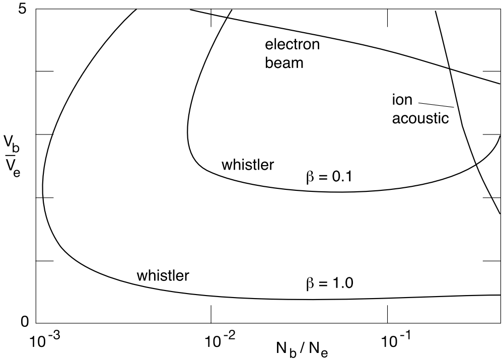
21.7 Shock Particle Reflection
The process of particle reflection from a shock wave is one of the most important processes in the entire physics of collisionless shocks. However, the mechanism of particle reflection has not yet been fully illuminated.
Particle reflection is caused by a combination of electrostatic and magnetic forces and is nearly specular in nature. It is required in supercritical shocks as it is the only process that can compensate for the incapability of dissipative processes inside the shock ramp to digest the fast inflow of momentum and energy into the shock. Shock particle reflection is not dissipative by itself even though in a fluid picture which deals with moments of the distribution function it can be interpreted as kind of an ion viscosity, i.e. it generates an anomalous viscosity coefficient which appears as a factor in front of the second derivative of the ion velocity in the ionic equation of motion. As such it also appears in the ion heat-transport equation. The kinematic ion viscosity can be expressed as \[ \mu_\mathrm{vis} = m_i n \nu_i \lambda_\mathrm{mfp} \simeq P_i / 2\omega_{ci} \] through the ion pressure \(P_i\) and the ion-cyclotron frequency \(\omega_{ci}\) when replacing the mean free path through the ion gyro-radius. In this sense shock particle reflection constitutes by itself a very efficient non-dissipative dissipation mechanism. However, its direct dissipative action is to produce real dissipation as far as possible upstream of the shock in order to dissipate as much energy of motion as remains to be in excess after formation of a shock ramp, dissipation inside the ramp, and reflection of ion back upstream. The shock does this by inhibiting a substantial fraction of inflow ions to pass across the shock from upstream into the downstream region. It is sending these ions back into the upstream region where they cause a violently unstable upstream ion beam-plasma configuration which excites a large amplitude turbulent wave spectrum that scatters the uninformed plasma inflow, heats it and retards it down to the Mach number range that can be digested by the shock. In this way the collisionless shock generates a shock transition region that extends far upstream with the shock ramp degrading to the role of playing a subshock at the location where the ultimate decrease of the Mach number from upstream to downstream takes place.
Shock reflection has another important effect on the shock as the momentum transfer from the reflected particle component to the shock retards the shock in the region of reflection thereby decreasing the effective Mach number of the shock.
21.7.1 Specular Reflection
Specular reflection of ions from a shock front, i.e. reversal of velocity normal component at the shock, is the simplest case to be imagined. It requires that the ions experience the shock ramp as an impenetrable wall. This can be the case when the shock itself contains a positive reflecting electric potential which builds up in front of the approaching ion. Generation of this electric potential is not clarified yet. In a very naive approach one assumes that in flowing magnetised plasma a potential wall is created as the consequence of charge separation between electrons and ions in penetrating the shock ramp. It occurs over a scale typically of the spatial difference between an ion and an electron gyro-radius, because in the ideal case the electrons, when running into the shock ramp, are held temporarily back in the steep magnetic field gradient over this distance while the ions feel the magnetic gradient only over a scale longer than their gyro-radius and thus penetrate deeper into the shock transition.
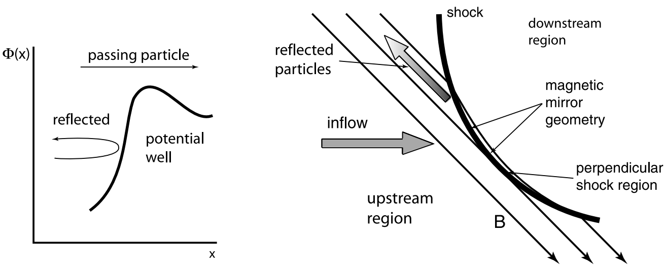
- Reflection from Shock Potential
Due to this simplistic picture the shock ramp should contain a steep increase in the electric potential \(\Delta\Phi\) which will reflect any ion which has less kinetic energy \(m_i V_N^2/2 < e\Delta\Phi\) (Figure 21.41).
- Mirror Reflection
Another simple possibility for particle reflection from a shock ramp in magnetised plasma is mirror reflection. An ion approaching the shock has components \(v_{i\parallel}\). Assume a curved shock like Earth’s bow shock. Close to its perpendicular part where the upstream magnetic field becomes tangential to the shock the particles approaching the shock with the stream and moving along the magnetic field with their parallel velocities experience a mirror magnetic field configuration that results from the converging magnetic field lines near the perpendicular point (Figure 21.41). Conservation of the magnetic moment \(\mu = T_{i\perp}/B\) implies that the particles become heated adiabatically in the increasing field; they also experience a reflecting mirror force \(-\mu \nabla_\parallel B\) which tries to keep ions away from entering the shock along the magnetic field. Particles will mirror at the perpendicular shock point and return upstream when their pitch angle becomes 90◦ at this location. (??? Leroy & Mangeney, 1984; Wu, 1984)
Specular reflection from shocks is the extreme case of shock particle reflection. Other mechanisms like turbulent reflection are, however, not well elaborated and must in any case be investigated with the help of numerical simulations.
21.7.2 Consequences of Shock Reflection
How far the reflected ions return upstream depends on the direction of the magnetic field with respect to the shock, i.e. on the shock normal angle \(\theta_{Bn}\). For perpendicular shocks the reflected ions only pass just one gyro-radius back upstream. Seeing the convection electric field \(\mathbf{E} = -\mathbf{v}_\mathrm{flow}\times\mathbf{B}\) they become accelerated along the shock forming a current, the velocity of which in any case exceeds the inflow velocity (which is zero in the perpendicular direction) and for sufficiently cold ions also the ion acoustic velocity \(c_{ia}\) in which case the ion-beam plasma instability will be excited in the shock foot region where the ion current flows. This may generate anomalous collision in the shock foot region. Moreover, since the excited waves accelerate electrons along the magnetic field other secondary instabilities can arise as well.
In quasi-perpendicular and oblique shocks the ions can escape along the magnetic field. In this case an ion two-stream situation arises between the upstream beam and the plasma inflow with the consequence of excitation of a variety of electromagnetic and electrostatic instabilities. In addition, however, an ion-electron two-stream situation is caused between the upstream ions and the inflow electrons which because of the large upstream electron temperatures probably excites mainly ion-acoustic modes but can also lead to Buneman two-stream mode excitation. These modes contribute to turbulence in the upstream foreshock region creating a weakly dissipative state in the foreshock where the plasma inflow becomes informed about the presence of the shock. The electromagnetic low frequency instabilities on the other hand, which are excited in this region, will grow to large amplitude, form localised structures and after being convected by the main flow towards the shock ramp interact with the shock and modify the shock profile or even contribute to shock formation and shock regeneration.
21.8 Shock Particle Acceleration
In the context of cosmic rays that have been observed in the interstellar space, medium energy particles refer to ~ few GeV ions and ~ few MeV electrons. Above these ranges relativistic shocks must be considered. Near the Earth’s bow shock the solar wind hydrogen kinetic energy is ~ 1 keV; ~ 10 keV is about the low threshold for energetic ions. Here we limit our discussions first to the non-relativistic case.
Figure 21.42 shows schematically the process of particle acceleration. Based on early estimations by Fermi (1949), a large number of shock crossings and reflections back and forth is required for the particles to reach energetic cosmic ray level. The scattering process is a stochastic process that is assumed to conserve energy; in particular they should not become involved into excitation of instabilities which consume part of their motional energy. The only actual dissipation that is allowed in this process is dissipation of bulk motional energy from where the few accelerated particles extract their energy gain. This dissipation is also attributed to direct particle loss by either convective transport or the limited size of the acceleration region. Thus this mechanism works until the gyro-radius of the accelerated particle becomes so large that it exceeds the size of the system.
The stochastic process implies that the basic equation that governs the process is a phase space diffusion equation in the form of a Fokker-Planck equation \[ \frac{\partial F(\mathbf{p}, \mathbf{x}, t)}{\partial t} + \mathbf{v}\cdot\nabla F(\mathbf{p},\mathbf{x},t) = \frac{\partial}{\partial \mathbf{p}}\cdot\mathbf{D}_{pp}\cdot\frac{\partial F(\mathbf{p}, \mathbf{x}, t)}{\partial \mathbf{p}},\quad \mathbf{D}_{pp}=\frac{1}{2}\left< \frac{\Delta \mathbf{p}\Delta \mathbf{p}}{\Delta t} \right> \] where \(\Delta \mathbf{p}\) is the variation of the particle momentum in the scattering process which happens in the time interval \(\Delta t\), and the angular brackets indicate ensemble averaging. \(\mathbf{D}_{pp}\) is the momentum space diffusion tensor. It is customary to define \(\mu = \cos\alpha\) as the cosine of the particle pitch angle \(\alpha\) and to understand among \(F(p,\mu)\) the gyro-phase averaged distribution function, which depends only on \(p = |\mathbf{p}|\) and \(\mu\).
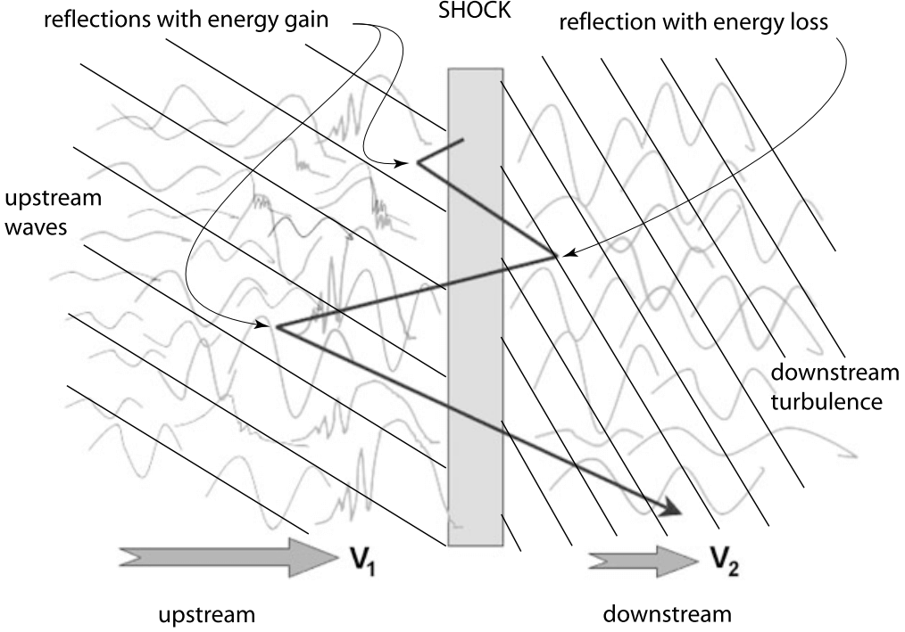
The dependence on the gyro-radius imposes a severe limitation on the acceleration mechanism, i.e. the injection problem. In order to experience a first scattering, i.e. in order to being admitted to the acceleration process, the particle must initially already possess a gyro-radius much larger than the entire width of the shock transition region. Only when this condition is given, the shock will behave like an infinitesimally thin discontinuity separating two regions of vastly different velocities such that the particle when crossing back and forth over the shock can become aware of the bulk difference in speed and take an energetic advantage of it. This restriction rules out any particles in the core of the upstream inflow distribution from participation in the acceleration process: in order to enter the Fermi shock-acceleration mechanism a particle must be pre-accelerated or pre-heated until its gyro-radius becomes sufficiently large. This condition poses the injection problem, where an unresolved seed population of energetic particles are needed for further acceleration, that has not yet been resolved.
Foreshock transients (Section 21.9), especially HFAs and FBs, can accelerate particles and contribute to the primary shock acceleration. These can form secondary shocks which leads to several possible acceleration mechanisms; they can also cause local magnetic reconnection that accelerate particles. The interaction with foreshock transients provides a possible solution to Fermi’s injection problem and increase the acceleration efficiency of primary shocks.
- As foreshock transients convect with the upstream flow, particles enclosed within their boundary and the primary shock can experience Fermi acceleration.
- Secondary shocks have also been observed to accelerate upstream particles on their own through the shock drift acceleration (SDA)28 and even to form a secondary foreshock.
- Secondary shocks can also capture and further energize primary shock-accelerated electrons through betatron acceleration.
- Magnetic reconnection inside foreshock transients contributes to the electron and ion acceleration/heating.
Another problem awakens attention is that how the shocks are modulated by the presence of energetic particles.
In terms of particle acceleration the shock appears as a boundary between two independent regions of different bulk flow parameters which are filled with scattering centres for the particles as sketched in Figure 21.43. Theoretically ((Balogh and Treumann 2013)) any particle which returns from downstream to upstream is accelerated in the upstream flow, even in the absence of any upstream turbulence and scatterings. If the upstream medium is magnetised and is sufficiently extended to host the upstream gyration orbit, pick-up ion energization can happen via the convection electric field \(\mathbf{E}=-\mathbf{V}\times\mathbf{B}\) all along their upstream half-gyrocircles. Alternatively, the upstream turbulence can also cause ion energization.
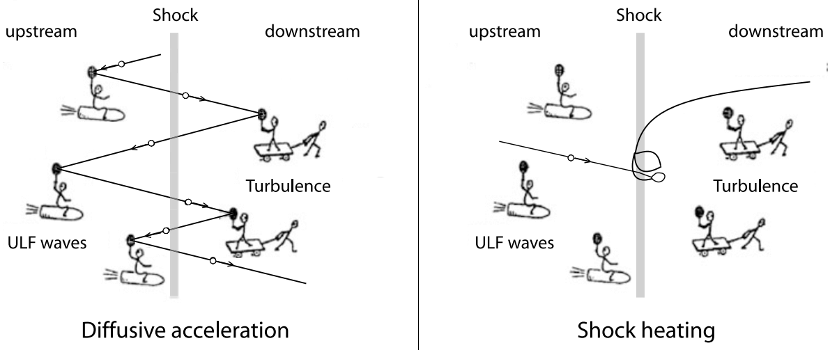
As a summary, diffusive shock acceleration (DSA) (1st-order Fermi acceleration) is the most widely accepted theory for particle acceleration for quasi-parallel shocks. However, a similar theory does not work efficiently at low energies at quasi-perpendicular shocks, where the reflected ions return to the shocks almost immediately due to their gyromotion in the upstream magnetic field. Therefore, shock drift acceleration (SDA) and shock surfing acceleration (SSA) are considered to play important roles in ion acceleration or pre-acceleration at quasi-perpendicular shocks.
21.8.1 Electron Acceleration and Heating at Shocks
For strong shocks with a quasiperpendicular geometry, while ion heating is commonly regarded as a result of particle reflection by electric and magnetic forces, the electron heating problem remains controversial. The key controversy concerning electron heating lies in how and when irreversible dissipation occurs. A widely accepted picture of electron heating at the Earth’s bow shock describes that the electron phase space is inflated by a quasistatic cross-shock potential accelerating (decelerating) incoming (escaping) electrons, conserving the first adiabatic invariant, and creates an inaccessible region at energies lower than the cross-shock potential energy of electrons [Schwartz 2012]. The inaccessible region is postulated to be filled by wave-particle scattering, leading to thermalization. The picture is based on past observations of heated “flat-topped” distributions and approximately isotropic temperature increase through the shock ramp.
Recent studies concern the breaking of adiabatic conditions (e.g. Li-jen Chen 2018 PRL). MMS observations show cases of bulk acceleration of the solar wind electrons and the nonlinear relaxation resulting in heating at a quasi-perpendicular shock front. The acceleration is achieved by an electric field embedded in a low-frequency whistler-mode wave, and leads to a high parallel current density. It is hypothesized that a collection of localized strong electric fields (\(E_n\) spikes, where n is the normal direction to the shock front) may constitute part of the “cross-shock potential”.
21.9 Foreshock Transients
This section provides a list and a very short description of foreshock transients based on observations including hot flow anomalies (HFAs), spontaneous hot flow anomalies (SHFAs), foreshock bubbles (FBs), foreshock cavities, foreshock cavitons, foreshock compressional boundaries, density holes, and Short Large-Amplitude Magnetic structures (SLAMs). Table 21.4 shows a comparison of their characteristics after (Zhang et al. 2022).
| Depletion in n and B | Compression in n and B | Presence of suprathermal ions | Flow deflection | Plasma heating | Associated with an IMF discontinuity | Duration | Scale size | ||
|---|---|---|---|---|---|---|---|---|---|
| HFA | Yes | At edges | Yes | Strong | Strong | Yes | \(10 - 10^2\) s | \(\mathcal{O}(R_E)\) | |
| SHFA | Yes | At edges | Yes | Strong | Strong | No | \(10 - 10^2\) s | \(\mathcal{O}(R_E)\) | |
| FB | Yes | Only on the upstream edge | Yes | Strong | Strong | Yes | \(10 - 10^2\) s | \(\mathcal{O}(R_E)\) | |
| Cavity | Yes | At edges | Yes | Weak | Modest | Sometimes | \(10 - 10^2\) s | \(\mathcal{O}(R_E)\) | |
| Caviton | Yes | At edges | Yes | Weak | Weak | No | \(10 - 60\) s | \(\mathcal{O}(R_E)\) | |
| FCB | Yes on the turbulent side | At edges | Maybe | Weak | Weak | No | \(10 - 10^2\) s | \(\mathcal{O}(R_E)\) | |
| Density Hole | Yes | At edges | Yes | Sometimes | Sometimes | Yes | \(1 - 60\) s | \(\mathcal{O}(R_E)\) | |
| SLAMS | No | Yes | Maybe | Sometimes | Sometimes | No | \(1 - 60\) s | \(<0.5\, R_E\) |
| Generation mechanism | |
|---|---|
| HFA | Interaction of IMF discontinuities with the bow shock |
| SHFA | Interaction of foreshock cavitons with the bow shock |
| FB | Kinetic interactions between suprathermal, backstreaming ions and incident SW plasma with embedded IMF discontinuities that move through and alter the ion foreshock |
| Cavity | Antisunward moving slabs of magnetic field lines that connect to the bow shock that are sandwiched between broader regions of magnetic field lines that remain unconnected to the bow shock |
| Caviton | Nonlinear interaction of ULF waves |
| FCB | Backstreaming ions result in increased pressure within the foreshock region leading to its expansion against the pristine SW and the generation of FCBs |
| Density Hole | Possibly due to backstreaming particles interacting with the original SW |
| SLAMS | Nonlinear wave steepening |
21.9.1 Hot Flow Anomaly
HFAs are characterized by a low field strength and low density core with heated plasma and substantial flow deflection with sizes of several \(\mathrm{R}_\mathrm{E}\). HFAs are typically driven by a solar wind tangential discontinuity (TD) that intersects the bow shock with solar wind convection electric field pointing inward on at least one side of the TD. Such a TD can locally trap foreshock ions leading to the HFA formation while propagating along the bow shock surface. HFAs may accelerate particles efficiently through Fermi acceleration, i.e., bouncing between the converging HFA boundary and the bow shock. The observed energetic ions may also have escaped from the outer magnetosphere.
One of the most remarkable properties of HFAs is the strong deflection of the solar wind bulk flow which can be large enough that inside an HFA the flow can actually show a sunward component. A transient region of lower density in the solar wind interacting with the fast shock can cause the disruption of the fast shock and leads to a new shock that actually travels into the upstream direction with plasma behind this new shock having a much smaller momentum density and velocity than the original solar wind.
21.9.2 Spontaneous Hot Flow Anomaly
SHFAs have the same characteristics as HFAs except that they are not associated with any solar wind discontinuities. They form intrinsically in the quasi-parallel regime, likely due to the interaction between foreshock cavitons and the bow shock.
In order to distinguish SHFAs from cavitons in simulations, an additional empirical criterion of SHFA having \(\beta > 10\) in at least 60% of the transient region has been used. It is chosen in order to not make assumptions on the level of heating and flow deflection inside the transients. A value of 10 indicates that the transients are dominated by the plasma instead of the magnetic field, and it is significantly above the typical β in the surrounding foreshock (\(β \sim 1-4\)).
21.9.3 Foreshock Bubble
When backstreaming foreshock ions interact with a solar wind rotational discontinuity (RD) that does not necessarily intersect the bow shock, FBs form upstream of the RD and convecting anti-sunward with it. Later observations and simulations found that TDs can also drive FBs. FBs are also characterized by a heated, tenuous core with significant flow deflection. Different from HFAs and SHFAs, the expansion of FBs is super-fast-magnetosonic and dominantly in the sunward direction. Because of the sunward super-fast-magnetosonic expansion, a shock forms upstream of the core, and the FB size in the expansion direction can reach 5-10 \(\mathrm{R}_\mathrm{E}\), larger than typical HFAs and SHFAs. In addition to their significant dynamic pressure perturbations, FBs are also efficient particle accelerators due to the presence of the shock (e.g., shock drift acceleration and Fermi acceleration as the shock converges towards the bow shock).
21.9.4 Foreshock Cavity
Foreshock cavities are characterized by low density, low field strength core regions with high density, high field strength compressional boundaries on two sides. But different from HFAs, the flow deflection inside foreshock cavities is rather weak and plasma heating is not significant. When slabs of magnetic field lines connected to the bow shock are bounded by broader regions of magnetic field lines that remain unconnected to the bow shock, only the slabs are filled with energized particles reflected from the bow shock. The presence of foreshock particles enhanced the thermal pressure, causing an expansion on two sides. Such an expansion decreases the plasma density and magnetic field strength inside the slabs and increases the density and field strength at two boundaries, i.e., a foreshock cavity forms.
Note that this is somehow different from another cavity known as the magnetic cavity, which is often interpreted as a magnetic mirror structure where a decrease in magnetic field at the center corresponds to an increase of particles at the center [J. Liu+ 2020].
21.9.5 Foreshock Caviton
Foreshock cavitons are also characterized by a core region with low density and field strength bounded by two boundaries with high density and field strength, without clear heating and flow deflection. Their sizes are about one \(\mathrm{R}_\mathrm{E}\). They form due to the nonlinear evolution of two types of waves: the parallel propagating right- or left-hand polarized waves and the obliquely propagating linearly polarized fast magnetosonic waves. Thus, foreshock cavitons are embedded in foreshock ULF waves, whereas foreshock cavities are isolated due to their different formation mechanisms.
21.9.6 Foreshock Compressional Boundary
FCBs have enhanced density and field strength. They occur at the boundary between the foreshock and the pristine solar wind. Because of the high thermal pressure due to the presence of foreshock ions, the foreshock region expands into the ambient pristine solar wind, leading to the formation of an FCB. FCBs are sometimes associated with local density and field strength depletion on their foreshock side. FCBs can form under either steady or nonsteady IMF conditions.
21.9.7 SLAMS and Shocklets
Short Large-Amplitude Magnetic Structures (SLAMS) are magnetic pulsations with amplitudes at least two times the ambient magnetic field strength. SLAMS have typical spatial scales up to many ion gyroradii (where the thermal ion gyroradius is typically 160 km in the solar wind) and grow rapidly with time scales of seconds. Shocklets are also magnetic structures (nonlinearly steepened magnetosonic waves), but differ from SLAMS in terms of amplitude, spatial scale, growth rate, and propagation angle.
21.9.8 Density Hole
Density holes are characterized by similarly shaped magnetic holes with enhanced density and field strength at one or both edges. The definition of density holes overlaps with HFAs, SHFAs, FBs, foreshock cavities, and foreshock cavitons, but in a broader sense. Lu et al. (2022) showed statistically that ∼66% of 411 density holes cannot be categorized by any of these foreshock transient types. Therefore, it is necessary to make density holes a separate category. A better definition of density holes is needed to definitely distinguish them from other foreshock transient types, which requires further studies. The formation could be due to the interaction between backstreaming particles and the original solar wind (Parks et al. 2006).
21.10 Location of Shocks
In the observation comparison paper (Slavin and Holzer 1981) for quasi-perpendicular shocks, they concluded that the variations in shock stand-off distance and shape are ordered by the sonic Mach number \(M_s\) and not other Mach numbers involve magnetic field. In other words, they think the bow shock is a gasdynamic structure.
However, even in neutral fluid theory, the determination of shock location as well as shape is still an ongoing research. Imagine the simplest scenario where there is a static ball in the air with infinite mass. Assuming purely homogenous air with known density, velocity and pressure in the upstream, can you tell me the exact location of shock stand-off distance with pen and paper?
On top of that, the introduction of EM field complicates the story. Especially in the case of a parallel shock, the plasmas get “shocked” both upstream and downstream, and the stand-off distance of the shock may not be a single point theoretically. In some sense, normal magnetic field to the boundary “thickens” the shock front.
21.11 Earth Bow Shock
Using data from the AMPTE/IRM spacecraft, (Hill et al. 1995) have shown that the double adiabatic equations do not hold in the magnetosheath. Moreover, the thermal behaviour of the magnetosheath is studied by (Phan et al. 1996) using WIND spacecraft data. They report that most parts of the magnetosheath are marginally mirror unstable: electron observations showed \(T_{e\perp} / T_{e\parallel} \sim 1.3\) in the magnetosheath.
One point that is probably confusing for many people is the difference between the ram pressure \(\rho U^2\) and the dynamic pressure \(\rho U^2/2\), which differs by a factor of 2. If the density is constant (which is a subset of incompressible fluid), the Bernoulli equation \(\rho V^2/2 + P_t + P_B = \text{const.}\) is satisfied. However, for compressible fluid the pressure balance equation is \(\rho V^2 + P_t + P_B = \text{const}\).↩︎
Fitzpatrick’s note use V for velocity. I prefer U for fluid velocities and V for particle velocities.↩︎
In aerodynamics, the critical Mach number \(M^\ast\) of an aircraft is the lowest Mach number at which the airflow over some point of the aircraft reaches the speed of sound, but does not exceed it. For an aircraft in flight, the speed of the airflow around the aircraft differs considerably in places from the airspeed of the aircraft; this is due to the airflow having to speed up and slow down as it travels around the aircraft’s structure. When the aircraft’s airspeed reaches the critical Mach number, the speed of the airflow in some areas near the airframe reaches the speed of sound, even though the aircraft itself has an airspeed lower than Mach 1.0. This creates a weak shock wave. As the aircraft exceeds the critical Mach number, its drag coefficient increases suddenly, causing dramatically increased drag, and may lead to deterioration in control of the aircraft.↩︎
so it depends on the upstream sound speed?↩︎
One way to define the tangential direction \(\hat{t}\) is to use \(\mathbf{U}_{t1}\) as a reference: \(\mathbf{U}_{t1} = \mathbf{U}_1 - (\mathbf{U}_1 \cdot \hat{n})\hat{n}\). Then \(\hat{t} = \mathbf{U}_{t1} / |\mathbf{U}_{t1}|\). Note that both the normal and tangential components are signed numbers.↩︎
The shock normal points from downstream to upstream, and the plasma flow points from upstream to downstream. Usually we take an angle smaller than \(90^\circ\), so the definition would be \(\theta_1 = \cos^{-1}(-\mathbf{U}_1 \cdot\hat{n}/|\mathbf{U}_1|)\).↩︎
Note that the velocity is defined in the dHT frame, not the lab frame! dHT is used here simply because the jump conditions are easier to solve. Also note that the jump conditions solved under the dHT frame is different from the lab frame!↩︎
This equation is only valid in the dHT frame. In the lab frame, there shall be another equation for solving the compression ratio r from upstream conditions. However, the two must give identical results for the uniqueness of shock.↩︎
This is a very strong indication that Alfvén waves are involved in switch-on/off shocks!↩︎
A finite initial phase \(\phi_0 = 0\) may, however, modify this conclusion shifting the boundary between quasi-parallel and quasi-perpendicular shock to angles larger or smaller than \(45^\circ\), depending on the sign of the initial phase.↩︎
This shock setup is common in local simulations, but is quite different from the global shock simulations. We are looking at new methods for setting up the local shock runs.↩︎
From our 1D simulations, the reflecting ratio is about 1%. I think it would be interesting to investigate why. The energy perspective is a good starting point.↩︎
Our chance may have arrived!↩︎
I have strong doubts here. According to my understanding, the authors support specular reflection in this case study!↩︎
It has been demonstrated by Yann using the hybrid Vlasov model Vlasiator.↩︎
This is something we can check with new simulations!↩︎
The diffusion coefficient has the correct dimension \(\text{m}^2\text{s}^{-1}\).↩︎
From the simulation perspective, it is also difficult to capture these high frequency waves. The best we can get for now is about up to 10 Hz.↩︎
Why are the electrons hot when \(T_e\) is much smaller than ion? Is the comparison based on speed?↩︎
A detailed overview of the early observations is given by Klimas [1985].↩︎
I think these reflecting wall setups are unrealistic!↩︎
It could (but is unlikely) also be generated by an anomalous collision frequency. This remains to be tested by further observations and data analysis.↩︎
Note that no resonant ion beam-whistler interaction exists as the beam is hot and diffuse.↩︎
If the typical Vlasiator simulation values are used, \(B=5\,\mathrm{nT}\), \(n=10^6/\mathrm{cc}\), \(v_A = 109\,\mathrm{km/s}\), \(\Delta v \sim 650\,\mathrm{km/s}\).↩︎
The statement in (Balogh and Treumann 2013) is hard to follow. Maybe what they tried to argue is that it is the perpendicular portion of the shock that creates these reflected ions and leads to the instability. Later in the book they argued that on a small scale quasi-parallel shocks become perpendicular.↩︎
so literally the Alfvénic branch?↩︎
In the early Vlasiator paper 2014, the simulated RH growth rate is lower than theory, even though in a 1D3V almost parallel configuration.↩︎
The essence of SDA is that the electric field increases in the middle of the shock! The linked animation shows a perpendicular shock scenario where SDA is not present if there is no increase of the electric field in the shock. However, the question remains: why does the electric field increase?↩︎