22  Magnetosphere

The big picture when considering the interaction of the solar wind and the magnetosphere is as follows:

1. Is there something that can penetrate from the solar wind into the magnetosphere?
2. Is there something that can be triggered from the interaction?
3. Is a physical process internally or externally driven?

22.1 Earth’s Magnetic Environment

In the first approximation the Earth’s magnetic field is that of a magnetic dipole (Section 3.8). The dipole axis is tilted 11◦ from the direction of the Earth’s rotation axis. The current circuit giving rise to the magnetic field is located in the liquid core about 1200–3400 km from the center of the planet. The current system is asymmetric displacing the dipole moment from the center, which together with inhomogeneous distribution of magnetic matter above the core gives rise to large deviations from the dipole field on the surface. The pure dipole field on the surface would be 30 µT at the dipole equator and 60 µT at the poles. However, the actual surface field exceeds 66 µT in the region between Australia and Antarctica and is weakest, about 22 µT, in a region called South Atlantic Anomaly (SAA).

22.1.1 Basic Structures

In the frame of reference of the Earth the solar wind is supermagnetosonic, exceeding the local magnetosonic speed \(v_ms = \sqrt{v_s^2 + v_A^2}\), where \(v_s\) is the sound speed, \(v_A\) is the Alfvén speed. Because fluid-scale perturbations cannot propagate faster than \(v_{ms}\), this leads to a formation of a collisionless shock front, called the bow shock, upstream of the magnetosphere. Under typical solar wind conditions the apex of the shock in the solar direction is about 3 \(R_E\) upstream of the magnetopause. The shock converts a considerable fraction of solar wind kinetic energy to heat and electromagnetic energy. The irregular shocked flow region between the bow shock and the magnetopause is called the magnetosheath.

22.1.2 The Dipole Field

The dipole field is an idealization where the source current is assumed to be confined into a point at the origin. The source of planetary and stellar dipoles is a finite, actually a large, current system within the celestial body. Such fields, including the Terrestrial magnetic field, are customarily represented as a multipole expansion: dipole, quadrupole, octupole, etc. When moving away from the source, the higher multipoles vanish faster than the dipole making the dipole field a good starting point to consider the motion of charged particles. In the dipole field charged particles behave adiabatically as long as their gyro radii are smaller than the gradient scale length of the field (Section 7.8) and their orbits are not disturbed by collisions or time-varying electromagnetic field.

For the geomagnetic field it is customary to define the spherical coordinates in a special way. The dipole moment (\(\mathbf{m}_\mathrm{E}\)) is in the origin and points approximately toward geographic south, tilted 11◦ as mentioned above. Similar to the geographic coordinates the latitude (\(\lambda\)) is zero at the dipole equator and increases toward the north, whereas the latitudes in the southern hemisphere are negative. The longitude (\(\phi\)) increases toward the east from a given reference longitude. In magnetospheric physics the longitude is often given as the magnetic local time (MLT). In the dipole approximation MLT is determined by the flare angle between two planes: the dipole meridional plane containing the subsolar point on the Earth’s surface, and the dipole meridional plane which contains a given point on the surface, i.e., the local dipole meridian. Magnetic noon (MLT = 12 h) points toward the Sun, midnight (MLT = 24 h) anti-sunward. Magnetic dawn (MLT = 6 h) is approximately in the direction of the Earth’s orbit around the Sun.

The SI-unit of \(m_\mathrm{E}\) is \(\mathrm{A}\, \mathrm{m}^2\). Sometimes it is convenient to replace \(m_\mathrm{E}\) by \(k_0 = \mu_0 m_\mathrm{E}/4\pi\), which is also customarily called dipole moment. The strength of the terrestrial dipole moment varies slowly. A sufficiently accurate approximation is \[ \begin{aligned} m_\mathrm{E} &= 8\times 10^{22}\, \mathrm{A}\,\mathrm{m}^2 \\ k_0 &= 8\times 10^{15}\, \mathrm{Wb}\,\mathrm{m}\, (\mathrm{SI}:\mathrm{Wb} = \mathrm{T}\,\mathrm{m}^2) \\ &= 8\times 10^{25}\,\mathrm{G}\,\mathrm{cm}^3\, (\mathrm{Gaussian units}, 1\,\mathrm{G}=10^{-4}\,\mathrm{T}) \\ &= 0.3\,\mathrm{G}\, R_\mathrm{E}^3\, (R_\mathrm{E}\simeq 6378\,\mathrm{km}) \end{aligned} \]

The last expression is convenient in practice because the dipole field on the surface of the Earth (at 1 \(R_\mathrm{E}\)) varies in the range 0.3–0.6 G.

Outside its source, the dipole field is a curl-free potential field \(\mathbf{B} = -\nabla\psi\), where the scalar potential is given by \[ \psi = -\mathbf{k}_0\cdot\nabla\frac{1}{r} = -k_0\frac{\sin\lambda}{r^2} \] yielding \[ \mathbf{B} = \frac{1}{r^3}\left[ 3(\mathbf{k}_0\cdot\hat{r})\hat{r} - \mathbf{k}_0 \right] \]

The components of the magnetic field are \[ \begin{aligned} B_r &= -\frac{2k_0}{r^3}\sin\lambda \\ B_\lambda &= \frac{k_0}{r^3}\cos\lambda \\ B_\phi &= 0 \end{aligned} \] and its magnitude is \[ B = \frac{k_0}{r^3}\left( 1+3\sin^2\lambda \right)^{1/2} \]

The equation of a magnetic field line is \[ r = r_0\cos^2\lambda \] where \(r_0\) is the distance where the field line crosses the equator. The length element of the magnetic field line element is \[ \mathrm{d}s = \left( \mathrm{d}r^2 + r^2\mathrm{d}\lambda^2 \right)^{1/2} = r_0\cos\lambda \left( 1+3\sin^2\lambda \right)^{1/2} \mathrm{d}\lambda \] This can be integrated in a closed form, yielding the length of the dipole field line \(S_d\) as a function of \(r_0\) \[ S_d \approx 2.7603 r_0 \tag{22.1}\]

The curvature radius \(RC = |\mathrm{d}^2\mathbf{r}/\mathrm{d}s^2|^{−1}\) of the magnetic field is an important parameter for the motion of charged particles. For the dipole field the radius of curvature is \[ R_c(\lambda) = \frac{r_0}{3}\cos\lambda \frac{\left( 1+3\sin^2\lambda \right)^{3/2}}{2-\cos^2\lambda} \]

Any dipole field line is determined by its (constant) longitude \(\phi_0\) and the distance where the field line crosses the dipole equator. This distance is often given in terms of the L-parameter \[ L = r_0 / R_E \tag{22.2}\]

For a given L the corresponding field line reaches the surface of the Earth at the (dipole) latitude \[ \lambda_e = \arccos\frac{1}{\sqrt{L}} \]

For example, L = 2 (the inner belt) intersects the surface at \(\lambda_e = 45^\circ\) , L = 4 (the heart of the outer belt) at \(\lambda_e = 60^\circ\) and L = 6.6 (the geostationary orbit) at \(\lambda_e = 67.1^\circ\).

The dipole field line length in Equation 22.1 was calculated from the dipole itself. Now we can calculate also the dipole field line length from a point on the surface to the surface on the opposite hemisphere to be \[ S_e \approx (2.7755 L - 2.1747) R_E \] which is a good approximation when \(L\gtrsim 2\).

The field magnitude along a given field line as a function of latitude is \[ B(\lambda) = \left[ B_r(\lambda)^2 + B_\lambda(\lambda)^2 \right]^{1/2} = \frac{k_0}{r_0^3}\frac{(1+3\sin^2\lambda)^{1/2}}{\cos^6\lambda} \]

For the Earth \[ \frac{k_0}{r_0^3} = \frac{0.3}{L}\,\mathrm{G} = \frac{3\times 10^{-5}}{L^3}\,\mathrm{T} \]

The actual geomagnetic field has considerable deviations from the dipolar field because the dipole is not quite in the center of the Earth, the source is not a point, and the electric conductivity of the Earth is not uniform. The geomagnetic field is described by the International Geomagnetic Reference Field (IGRF) model, which is regularly updated to reflect the slow secular variations of the field, i.e., changes in timescales of years or longer.

22.1.3 Current Systems

The Earth’s magnetosphere is the region where the near-Earth magnetic field controls the motion of charged particles. It is formed by the interaction between the geodipole and the solar wind. The deformation of the field, caused by the variable solar wind pressure, sets up time-dependent magnetospheric current systems that dominate deviations from the dipole field in the outer radiation belt and beyond.

The solar wind plasma cannot easily penetrate to the Earth’s magnetic field and the outer magnetosphere is essentially a cavity around which the solar wind flows. The cavity is bounded by a flow discontinuity called the magnetopause. The shape and location of the magnetopause is determined by the balance between the solar wind plasma pressure and the magnetospheric magnetic field pressure. The nose, or apex, of the magnetopause is, under average solar wind conditions, at the distance of about 10 \(R_E\) from the center of the Earth but can be pushed to the vicinity of the geostationary distance (6.6 \(R_E\)) during periods of large solar wind pressure. In the dayside the dipole field is compressed toward the Earth, whereas in the nightside the field is stretched to form a long magnetotail. The deviations from the curl-free dipole field correspond to electric current systems according to Ampère’s law \(\mathbf{J}=\nabla\times\mathbf{B}/\mu_0\).

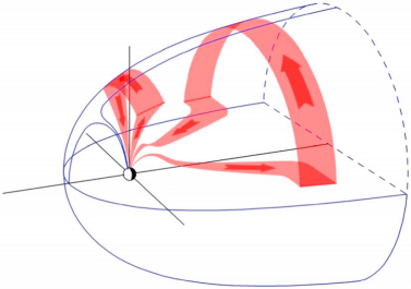
Figure 22.1 is a sketch of the magnetosphere with the main large-scale magnetospheric current systems. Individual looks at different currents in detail are presented in Figure 22.4, Figure 22.5, and Figure 22.6, with more explanations in this review.

Figure 22.1: The magnetosphere and the large scale magnetospheric current systems.

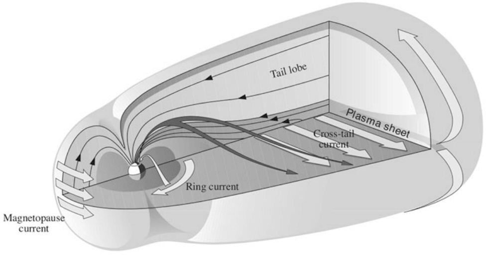
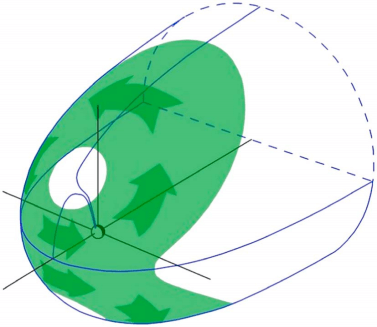
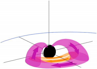
The current system on the dayside magnetopause shielding the Earth’s magnetic field from the solar wind is known as the Chapman–Ferraro current (Figure 22.2). In the first approximation the Chapman–Ferraro current density \(\mathbf{J}_\mathrm{CF}\) can be expressed as \[ \mathbf{J}_\mathrm{CF} = \frac{\mathbf{B}_\mathrm{MS}}{B_\mathrm{MS}^2}\times\nabla P_\mathrm{dyn} \tag{22.3}\] where \(\mathbf{B}_\mathrm{MS}\) is the magnetospheric magnetic field and \(P_\mathrm{dyn}\) the dynamic pressure of the solar wind. Because the interplanetary magnetic field (IMF) at the Earth’s orbit is only a few nanoteslas, the magnetopause current must shield the magnetospheric field to almost zero just outside the current layer. Consequently, the magnetic field immediately inside the magnetopause doubles: about one half comes from the Earth’s dipole and the second half from the magnetopause current. In plasma physics this is known as the diamagnetic current caused by the pressure gradient (Equation 8.63, Equation 8.65).

Figure 22.2: The Chapman-Ferraro dayside magnetopause currents are shown as a green-shaded surface on a simple wire diagram of the magnetopause. The Earth is the small sphere at the axis origin, and the Sun is to the lower left.

If the plasma pressure is anisotropic, the current density perpendicular to the magnetic field \(\mathbf{J}_\perp\) in a static system can be written \[ \mathbf{J}_\perp = \frac{\mathbf{B}}{B^2}\times\left[ \nabla p_\perp + (p_\parallel - p_\perp)\frac{(\mathbf{B}\cdot\nabla)\mathbf{B}}{B^2} \right] \tag{22.4}\] where \(p_\parallel\) and \(p_\perp\) are plasma pressure, parallel and perpendicular to the magnetic field, respectively. Equation 22.4 can be simplified to Equation 22.3 in the isotropic case.

The Chapman–Ferraro model describes a teardrop-like closed magnetosphere that is compressed in the dayside and stretched in the nightside, but not very far. Since the 1960s spacecraft observations have shown that the nightside magnetosphere, the magnetotail, is very long, extending far beyond the orbit of the Moon. This requires a mechanism to transfer energy from the solar wind into the magnetosphere to keep up the current system that sustains the tail-like configuration.

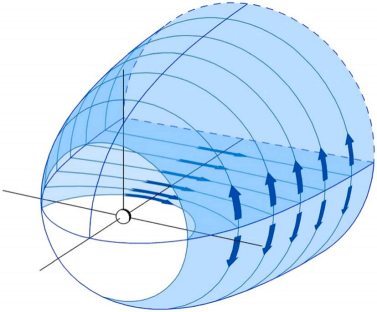
In Figure 22.1, the overwhelming fraction of the magnetospheric volume consists of tail lobes, connected magnetically to the polar caps in the ionized upper atmosphere, known as the ionosphere. The polar caps are bounded by auroral ovals. Consequently, in the northern lobe the magnetic field points toward the Earth, in the southern away from the Earth. To maintain the lobe structure, there must be a current sheet between the lobes where the current points from dawn to dusk. This cross-tail current is embedded within the plasma sheet and closes around the tail lobes forming the nightside part of the the magnetopause current.

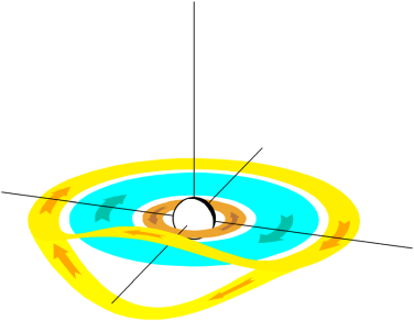
The cusp-like configurations of weak magnetic field above the polar regions known as polar cusps do not connect magnetically to magnetic poles, but instead to the southern and northern auroral ovals at noon, because the entire magnetic flux enclosed by the ovals is connected to the tail lobes. Tailward of the cusps the Chapman–Ferraro current and the tail magnetopause current smoothly merge with each other. Figure 22.1 also illustrates the westward flowing ring current (RC) and the magnetic field-aligned currents (FAC) connecting the magnetospheric currents to the horizontal ionospheric currents in auroral regions at an altitude of about 100 km. FACs are mainly carried by electrons. They were first suggested to explain the variations of magnetic field measured on the ground in the polar regions.

Figure 22.3: The tail current with closure via return current on magnetopause shown in light blue on the wire diagram of the magnetopause, as in Figure 22.2.

Figure 22.4: The symmetric ring current (eastward and westward, in brown and blue, respectively) including the cut ring currents on the dayside (in yellow). The viewing perspective is the same as in Figure 22.2 but now zoomed in closer to the Earth.

Figure 22.5: Region 1 field-aligned currents, shown as the red bands, including the two possible closure paths: directly to the magnetopause and via the far tail plasma sheet.

Figure 22.6: Region 2 field-aligned currents and partial ring current, shown in purple and the banana current, shown in orange. The view here is shifted to be from the evening sector.

Based on the magnetosphere-ionosphere current continuity, the field-aligned current \(J_\parallel\) (positive if flowing into the ionosphere) is related to the magnetic field and plasma pressure in the magnetosphere (Grad, 1964; Tverskoy, 1982; Vasyliunas, 1970) as (???) \[ J_\parallel = \frac{B_i}{B_e}\hat{b}\cdot\left( \nabla W \times \nabla P \right) \tag{22.5}\] where \(W = \int \frac{\mathrm{d}s}{B}\) is the magnetic flux tube volume, \(\mathrm{d}s\) is the element of magnetic field line length, \(B\) is the magnetic field along the field line and the integration is taken between the two conjugate points, \(P\) is the plasma pressure, \(B_i\) and \(B_e\) are the magnetic fields in the ionosphere and equatorial plane, respectively. The gradients are evaluated in the equatorial plane. The formation of a FAC requires the existence of a hot plasma pressure gradient along the isosurfaces of the magnetic flux tube volume W, azimuthal plasma pressure gradient. If the azimuthal gradient is directed outward indicating that the pressure peaks are not around midnight but close to dawn and dusk, Region 1 field-aligned current can be generated in the plasma sheet, as shown in Figure 22.5.

The magnetospheric current systems can have significant temporal variations, which makes the mathematical description of the magnetic field complicated. A common approach is to apply some of the various models developed by Nikolai Tsyganenko (Tsyganenko 2013).¹

For illustrative purposes simpler models are sometimes useful. For example, the early time-independent model of Mead (1964) reduces in the magnetic equatorial \((r, \phi)\) plane to \[ B(r,\phi) = B_E\left( \frac{R_E}{r} \right)^3 \left[ 1 + \frac{b_1}{B_E}\left( \frac{r}{R_E} \right)^3 - \frac{b_2}{B_E}\left( \frac{r}{R_E} \right)^4 \cos\phi \right] \] where \(B_E\) is the equatorial dipole field on the surface of the Earth (approximately 30.4 µT = 30,400 nT) and φ is the longitude east of midnight. The \(\cos\phi\) term describes the azimuthal asymmetry due to the dayside compression and nightside stretching of the field. The coefficients \(b_1\) and \(b_2\) depend on the distance of the subsolar point of the magnetopause \(R_s\) (in units of \(R_E\)), which, in turn, depends on the upstream solar wind pressure \[ \begin{aligned} b_1 &= 25\left( \frac{10}{R_s} \right)^3\,\mathrm{nT} \\ b_2 &= 2.1\left( \frac{10}{R_s} \right)^4\,\mathrm{nT} \end{aligned} \]

This model is fairly accurate during quiet and moderately disturbed times at geocentric distances 1.5–7 \(R_E\).

22.1.4 Geomagnetic Activity Indices

The intensity and variations of magnetospheric and ionospheric current systems are traditionally described in terms of geomagnetic activity indices. The indices are calculated from ground-based magnetometer measurements. As different indices describe different features of magnetospheric currents, there is no one-to-one correspondence between them. The choice of a particular index depends on physical processes being investigated.

The most widely used indices for global storm levels are Dst, Kp, and AE.

22.1.4.1 Dst

The Dst index aims at measuring the intensity of the ring current. It is calculated once an hour as a weighted average of the deviation from the quiet level of the horizontal magnetic field component (H) measured at four low-latitude stations distributed around the globe. Geomagnetic storms are defined as periods of strongly negative Dst index, signalling enhanced westward the ring current. The more negative the Dst index is, the stronger is the storm. There is no canonical lower threshold for the magnetic perturbation beyond which the state of the magnetosphere is to be called a storm and identification of weak storms is often ambiguous. As an empirical classification, we call storms with Dst from –50 to –100 nT moderate, from –100 to –200 nT intense, and those with Dst < −200 nT big. A similar 1-min index derived from a partly different set of six low-latitude stations (SYM–H) is also in use.

Dst has contributions from all currents in addition to the ring current. These include the magnetopause and cross-tail currents, as well as induced currents in the ground due to rapid temporal changes of ionospheric currents. Large solar wind pressure pushes the magnetopause closer to the Earth forcing the magnetopause current to increase to be able to shield a locally stronger geomagnetic field from the solar wind. The effect is strongest on the dayside where the magnetopause current flows in the direction opposite to the ring current. The pressure corrected Dst index can be defined as \[ \mathrm{Dst}^\ast = \mathrm{Dst} - b\sqrt{P_\mathrm{dyn}} + c \tag{22.6}\] where \(P_\mathrm{dyn}\) is the solar wind dynamic pressure and b and c are empirical parameters, whose exact values depend on the used statistical analysis methods, e.g., \(b = 7.26\,\mathrm{nT}\,\mathrm{nPa}^{−1/2}\) and \(c = 11\,\mathrm{nT}\) as determined by O’Brien and McPherron (2000).

The contribution from the dawn-to-dusk directed tail current to the Dst index is more difficult to estimate. During strong activity the cross-tail current intensifies and moves closer to the Earth, enhancing the nightside contribution to Dst. The estimates of this effect on Dst vary in the range 25–50%. Furthermore, fast temporal changes in the ionospheric currents induce strong localized currents in the ground, which may contribute up to 25% to the Dst index.

22.1.4.2 Kp

Another widely used index is the planetary K index, Kp. Each magnetic observatory has its own K index and Kp is an average of K indices from 13 mid-latitude stations. It is a quasi-logarithmic range index expressed in a scale of one-thirds: 0, 0+, 1−, 1, 1+,…, 8+, 9−, 9. Kp is based on mid-latitude observations and thus more sensitive to high-latitude auroral current systems and to substorm activity than the Dst index. Kp is a 3-h index and does not reflect rapid changes in the magnetospheric currents.

22.1.4.3 AE

The fastest variations in the current systems take place at auroral latitudes. To describe the strength of the auroral currents the auroral electrojet indices (AE) are commonly used. The standard AE index is calculated from 11 or 12 magnetometer stations located under the average auroral oval in the northern hemisphere. It is derived from the magnetic north component at each station by determining the envelope of the largest negative deviation from the quiet time background, called the AL index, and the largest positive deviation, called the AU index. The AE index itself is \(\mathrm{AE} = \mathrm{AU} - \mathrm{AL}\) (all in nT). Thus AL is the measure of the strongest westward current in the auroral oval, AU is the measure of the strongest eastward current, and AE characterizes the total electrojet activity. AE, AU, AL are typically given with 1-min time resolution.

As the auroral electrojets flow at the altitude of about 100 km, their magnetic deviations on the ground are much larger than those caused by the ring current. For example, during typical substorm activations AE is in the range 200–400 nT and can during strong storms exceed 2000 nT, whereas the equatorial Dst perturbations exceed −200 nT only during the strongest storms.

22.2 Particles

Typical densities of the unperturbed solar wind at 1 AU extend from about \(3\,\mathrm{cm}^{-3}\) in the fast (\(\sim 750\,\mathrm{km}\,\mathrm{s}^{-1}\)) to about \(10\,\mathrm{cm}^{-3}\) in the slow (\(\sim 350\,\mathrm{km}\,\mathrm{s}^{-1}\)) solar wind, again with large deviations.

22.2.1 Outer Magnetosphere

The outer magnetosphere can be considered to begin at distances of about 7–8 \(R_E\) where the nightside magnetic field becomes increasingly stretched. Table 22.1 summarizes typical plasma parameters in the mid-tail region, at about \(X = -20\, R_E\) from the Earth. Here \(X\) is the Earth-centered coordinate along the Earth–Sun line, positive toward the Sun. The tail lobes are almost empty, particle number densities being of the order of 0.01 \(\mathrm{cm}^{-3}\). The central plasma sheet where the cross-tail current is embedded (Figure 22.1) is, in turn, a region of hot high-density plasma. It is surrounded by the plasma sheet boundary layer with density and temperature intermediate to values in the central plasma sheet and tail lobes. The field lines of the boundary layer connect to the poleward edge of the auroral oval. The actual numbers differ considerably from the typical values under changing solar wind conditions and, in particular, during strong magnetospheric disturbances.

Table 22.1: Typical values of plasma parameters in the mid-tail

	Magnetosheath	Tail lobe	Plasma sheet boundary	Central plasma sheet
\(n(\mathrm{cm}^{-3})\)	8	0.01	0.1	0.3
\(T_i(\mathrm{eV})\)	150	300	1000	4200
\(T_e(\mathrm{eV})\)	25	50	150	600
\(B(\mathrm{nT})\)	15	20	20	10
\(\beta\)	2.5	0.0003	0.1	6

Table 22.1 also includes typical parameters in the magnetosheath at the same X-coordinate. The magnetosheath consists of solar wind plasma that has been compressed and heated by the Earth’s bow shock. It has higher density and lower temperature than observed in the outer magnetosphere. Table 22.1 shows that, while the magnetic field magnitude is rather similar in all regions shown, plasma beta (the ratio between the kinetic and magnetic field pressures), is a useful parameter to distinguish between different regions.

22.2.2 Inner Magnetosphere

The inner magnetosphere is the region where the magnetic field is quasi-dipolar. It is populated by different spatially overlapping particle species with different origins and widely different energies: the ring current, the radiation belts and the plasmasphere (Chapter 24). The ring current and radiation belts consist mainly of trapped particles in the quasi-dipolar field drifting due to magnetic field gradient and curvature effects around the Earth, whereas the motion and spatial extent of plasmaspheric plasma is mostly influenced by the corotation and convection electric fields.

The ring current arises from the azimuthal drift of energetic charged particles around the Earth; positively charged particles drifting toward the west and electrons toward the east. Basically all drifting particles contribute to the ring current. The drift currents are proportional to the energy density of the particles and the main ring current carriers are positive ions in the energy range 10–200 keV, whose fluxes are much larger than those of the higher-energy radiation belt particles. The ring current flows at geocentric distances 3–8 \(R_E\), and peaks at about 3–4 \(R_E\). At the earthward edge of the ring current the negative pressure gradient introduces a local eastward diamagnetic current, but the net current remains westward.

During magnetospheric activity the role of the ionosphere as the plasma source of ring current enhances, increasing the relative abundance of oxygen (\(\mathrm{O}^+\)) and helium (\(\mathrm{He}^+\)) ions in the magnetosphere. As a result a significant fraction of ring current can at times be carried by oxygen ions of atmospheric origin. The heavy-ion content furthermore modifies the properties of plasma waves in the inner magnetosphere, which has consequences on the wave–particle interactions with the radiation belt electrons.

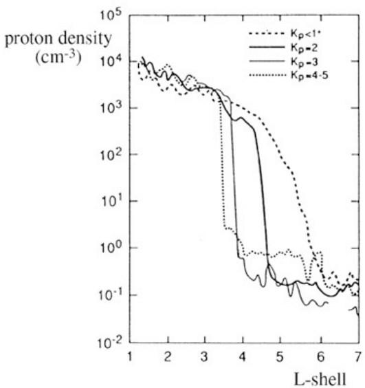
The plasmasphere is the innermost part of the magnetosphere. It consists of cold (\(\sim 1\,\mathrm{eV}\)) and dense (\(\gtrsim 10^3\, \mathrm{cm}^{-3}\)) plasma of ionospheric origin. The existence of the plasmasphere was already known before the spaceflight era based on the propagation characteristics of lightning-generated and man-made very low-frequency (VLF) waves. The plasmasphere has a relatively clear outer edge, the plasmapause, where the proton density drops several orders of magnitude. The location and structure of the plasmapause vary considerably as a function of magnetic activity (Figure 22.7). During magnetospheric quiescence the density decreases smoothly at distances from 4–6 \(R_E\), whereas during strong activity the plasmapause is steeper and pushed closer to the Earth.

Figure 22.7: Plasma density in the night sector organized by the activity index Kp. Kp < 1+ corresponds to a very quiet magnetosphere, whereas Kp = 4-5 indicates a significant activity level, although not yet a big magnetic storm. The L-shell is defined in Equation 22.2. [Chappell (1972)]

The location of the plasmapause is determined by the interplay between the sunward convection of plasma sheet particles and the plasmaspheric plasma corotating with the Earth. By adding the convective and corotational electric fields to the guiding center motion of charged particles we find that an outward bulge called plasmaspheric plume develops on the duskside around 18 h magnetic local time (MLT). Plasmaspheric plumes are most common and pronounced during geomagnetic storms and substorms, but they can exist also during quiet conditions (e.g., Moldwin+ 2016). During geomagnetic storms the plume can expand out to geostationary orbit and bend toward earlier MLT.

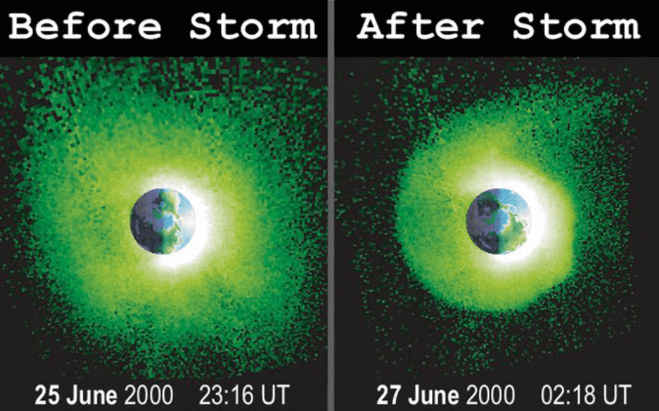
Figure 24.3 shows global observations of the plasmasphere taken by the EUV instrument onboard the IMAGE satellite before and after a moderate geomagnetic storm in June 2000. Before the storm the plasmasphere was more or less symmetric. After the storm the plasmasphere was significantly eroded leaving a plume extending from the dusk toward the dayside magnetopause. When traversing the plume, the trapped radiation belt electrons, otherwise outside the plasmapause, encounter a colder and higher-density plasma with plasma wave environment similar to the plasmasphere proper. Consequently, the influence of the plasmasphere on radiation belt particles extends beyond its nominal boundary depicted in Figure 22.7.

Figure 22.8: Plasmapheric plume and plasmaspheric erosion as observed by the IMAGE EUV instrument. The picture is taken from above the northern hemisphere and the Sun is to the right. (Goldstein+2004)

The plasma parameters in the plasmasphere, in the plume and at the plasmapause are critical to the generation and propagation of plasma waves that, in turn, interact with the energetic particles in the ring current and radiation belts. Thus, the coldest and the hottest components of the inner magnetosphere are intimately coupled to each other through wave–particle interactions.

It is important to recognize that the ring current is the main driver of the field perturbations, whereas the radiation belt has negligible contributions due to its low number density.

22.2.3 Cosmic Rays

In addition to ion and electron radiation belts another important component of corpuscular radiation in the near-Earth space consists of cosmic rays. The kinetic energies of a large fraction of cosmic ray particles are so large that the geomagnetic field cannot trap them. Instead, the particles traverse through the Earth’s magnetosphere without much deflection of their trajectories. Some of them hit the atmosphere interacting with nuclei of atmospheric atoms and molecules causing showers of elementary particles being possible to detect on ground. Those with highest energies can penetrate all the way to the ground.

The spectrum of cosmic ray ions at energies below about \(10^{15}\) eV per nucleon in the near-Earth space has three main components:

• Galactic cosmic rays (GCR), whose spectrum peaks at energies above 100 MeV per nucleon, are most likely accelerated by supernova remnant shock waves in our galaxy.
• Solar cosmic rays (SCR) are accelerated by coronal and interplanetary shocks related to solar eruptions. Their energies are mostly below 100 MeV per nucleon and a fraction of them can become trapped in the inner radiation belt.
• Anomalous cosmic rays (ACR) are ions of solar origin captured and accelerated by the heliospheric termination shock, where the supersonic solar wind becomes subsonic before encountering the interstellar plasma, or in the heliosheath outside the heliopause. Some of the ions are injected back toward the Sun. Near the Earth the ACR spectrum peaks at about 10 MeV per nucleon and thus the particles can become trapped in the geomagnetic field.

Although the galactic cosmic rays cannot directly be trapped into the radiation belts, they contribute indirectly to the inner belt composition through the Cosmic Ray Albedo Neutron Decay (GRAND) mechanism. The cosmic ray bombardment of the atmosphere produces neutrons that move in all directions. Although the average neutron lifetime is 14 min 38 s, during which a multi-MeV neutron either hits the Earth or escapes far away from the magnetosphere, a small fraction of them decay to protons while still in the inner magnetosphere and may become trapped in the inner radiation belt.

Below about 10 GeV GCR and ACR fluxes are modulated by the 11- and 22-year solar cycles, so they provide quasi-stationary background radiation in the timescales of radiation belt observations. The arrivals of SCRs are, in turn, transient phenomena related to solar flares and coronal mass ejections.

The cosmic ray electrons also have galactic and solar components. Furthermore, the magnetosphere of Jupiter accelerates high-energy electrons escaping to the interplanetary space. These Jovian electrons can be observed near the Earth at intervals of about 13 months when the Earth and Jupiter are connected by the IMF.

Supernova shock waves are the most likely sources of the accelerated GCR electrons, whereas in the acceleration of SCR and Jovian electrons also other mechanisms besides shock acceleration are important, in particular inductive electric fields associated with magnetic reconnection in solar flares and the Jovian magnetosphere.

The acceleration and identity of the observed very highest-energy cosmic rays up to about \(3\times 10^{20}\) eV remain enigmatic. It should not be possible to observe protons with energies higher than \(6\times 10^{19}\) eV, known as the Greisen–Zatsepin–Kuzmin cutoff, unless they are accelerated not too far from the observing site. Above the cutoff the interaction of protons with the blue-shifted cosmic microwave background produces pions that carry away the excessive energy. It is possible that the highest-energy particles are nuclei of heavier elements. This is, for the time being, an open question.

22.3 Magnetospheric Dynamics

Strong solar wind forcing drives storms and more intermittent substorms in the magnetosphere. They are primarily caused by various large-scale heliospheric structures such as interplanetary counterparts of coronal mass ejections (CMEs/ICMEs)², stream interaction regions (SIRs) of slow and fast solar wind flows, and fast solar wind supporting Alfvénic fluctuations. ICMEs are often preceded by interplanetary fast forward shocks and turbulent sheath regions between the shock and the ejecta, which all create their distinct responses in the magnetosphere. Because fast solar wind streams originate from coronal holes, which can persist over several solar rotations, the slow and fast stream pattern repeats in 27-day intervals and SIRs are often called co-rotating interaction regions (CIRs). However, stream interaction region is a physically more descriptive term. SIRs may gradually evolve to become bounded by shocks, but fully developed SIR shocks are only seldom observed sunward of the Earth’s orbit. The duration of these large-scale heliospheric structures near the orbit of the Earth varies from a few hours to days. On average, the passage of a sheath region past the Earth takes 8–9 h and the passage of an ICME or SIR about 1 day. The fast streams typically influence the Earth’s environment for several days.

22.3.1 Magnetospheric Convection

Magnetospheric plasma is in a continuous large-scale advective motion, which in this context is, somewhat inaccurately, called magnetospheric convection. The convection is most directly observable in the polar ionosphere, where the plasma flows from the dayside across the polar cap to the nightside and turns back to the dayside through the morning and evening sector auroral region. The non-resistive ideal magnetohydrodynamics (MHD) is a fairly accurate description of the large-scale plasma motion above the resistive ionosphere. In ideal MHD the magnetic field lines are electric equipotentials and the electric field \(\mathbf{E}\) and plasma velocity \(\mathbf{V}\) are related to each other through the simple relation \[ \mathbf{E} = -\mathbf{V}\times\mathbf{B} \]

Consequently, the observable convective motion, or alternatively the electric potential, in the ionosphere can be mapped along the magnetic field lines to plasma motion in the tail lobes and the plasma sheet. As the electric field in the tail plasma sheet points from dawn to dusk and the magnetic field to the north, the convection brings plasma particles from the nightside plasma sheet toward the Earth where a fraction of them become carriers of the ring current and form the source population for the radiation belts.

In ideal MHD the plasma and the magnetic field lines are said to be frozen-in to each other. This means that two plasma elements that are connected by a magnetic field line remain so when plasma flows from one place to another. It is convenient to illustrate the motion with moving field lines, although the magnetic field lines are not physical entities and their motion is just a convenient metaphor. A more physical description is that the magnetic field evolves in space and time such that the plasma elements maintain their magnetic connection.

The convection is sustained by solar wind energy input into the magnetosphere. The input is weakest, but yet finite, when the interplanetary magnetic field (IMF) points toward the north, and is enhanced during southward pointing IMF. If the magnetopause were fully closed, plasma would circulate inside the magnetosphere so that the magnetic flux tubes crossing the polar cap from dayside to nightside would reach to the outer boundary of the magnetosphere where some type of viscous interaction with the anti-sunward solar wind flow would be needed to maintain the circulation. The classical (collisional) viscosity on the magnetopause is vanishingly small, but finite gyro radius effects and wave–particle interactions give rise to some level of anomalous viscosity³. It is estimated to provide about 10% of the momentum transfer from the solar wind to the magnetosphere.

The magnetosphere is, however, not fully closed. In the same year, when Axford and Hines presented their viscous interaction model, Dungey (1961) explained the convection in terms of magnetic reconnection. The Dungey cycle begins with a violation of the frozen-in condition at the dayside magnetopause current sheet. A magnetic field line in the solar wind is cut and reconnected with a terrestrial field line. Reconnection is most efficient for oppositely directed magnetic fields, as is the case in the dayside equatorial plane when the IMF points southward, but remains finite under other orientations. Subsequent to the dayside reconnection the solar wind flow drags the newly-connected field line to the nightside and the part of the field line that is inside the magnetosphere becomes a tail lobe field line. Consequently, an increasing amount of magnetic flux is piling up in the lobes. At some distance far in the tail the oppositely directed field lines in the northern and southern lobes reconnect again across the cross-tail current layer. At this point the ionospheric end of the field line has reached the auroral oval near local midnight. Now the earthward outflow from the reconnection site in the tail drags the newly-closed field line toward the Earth. The return flow cannot penetrate to the plasmasphere corotating with the Earth and the convective flow must proceed via the dawn and dusk sectors around the Earth to the dayside. In the ionosphere the flow returns toward the dayside along the dawnside and duskside auroral oval. Once approaching the dayside magnetopause, the magnetospheric plasma provides the inflow to the dayside reconnection inside of the magnetopause. Note that the resistive ionosphere breaks the frozen-in condition of ideal MHD and it is not reasonable to use the picture of moving field lines in the atmosphere.

The increase in the tail lobe magnetic flux and strengthening of plasma convection inside the magnetosphere during southward IMF have a strong observational basis. Calculating the east-west component of the motion-induced solar wind electric field (\(E = V\, B_\mathrm{south}\)) incident on the magnetopause and estimating the corresponding potential drop over the magnetosphere, some 10% of the solar wind electric field is estimated to “penetrate” into the magnetosphere as the dawn-to-dusk directed convection electric field. Note that \(\mathbf{E} = -\mathbf{V}\times\mathbf{B}\) is not a causal relationship indicating whether it is the electric field that drives the magnetospheric convection, or convection that gives rise to the motion-induced electric field. The ultimate driver of the circulation is the solar wind forcing on the magnetosphere.

The plasma circulation is not as smooth as the above discussion may suggest. If the reconnection rates at the dayside magnetopause and nightside current sheet balance each other, a steady-state convection can, indeed, arise. This is, however, seldom the case since the changes in the driving solar wind and in the magnetospheric response are faster than the magnetospheric circulation timescale of a few hours. Reconnection may cause significant erosion of the dayside magnetospheric magnetic field placing the magnetopause closer to the Earth than a simple pressure balance consideration would indicate. The changing magnetic flux in the tail lobes causes expansion and contraction of the polar caps affecting the size and shape of the auroral ovals.

Furthermore, the convection in the plasma sheet has been found to consist of intermittent high-speed bursty bulk flows (BBF) with almost stagnant plasma in between (Angelopoulos et al. 1992). It is noteworthy that while BBFs are more frequent during high auroral activity, they also appear during auroral quiescence. BBFs have been estimated to be the primary mechanism of earthward mass and energy transport in regions where they have been observed. Thus the high-latitude convection observed in the ionosphere corresponds to an average of the BBFs and slower background flows in the outer magnetosphere.

22.3.2 Geomagnetic Storms

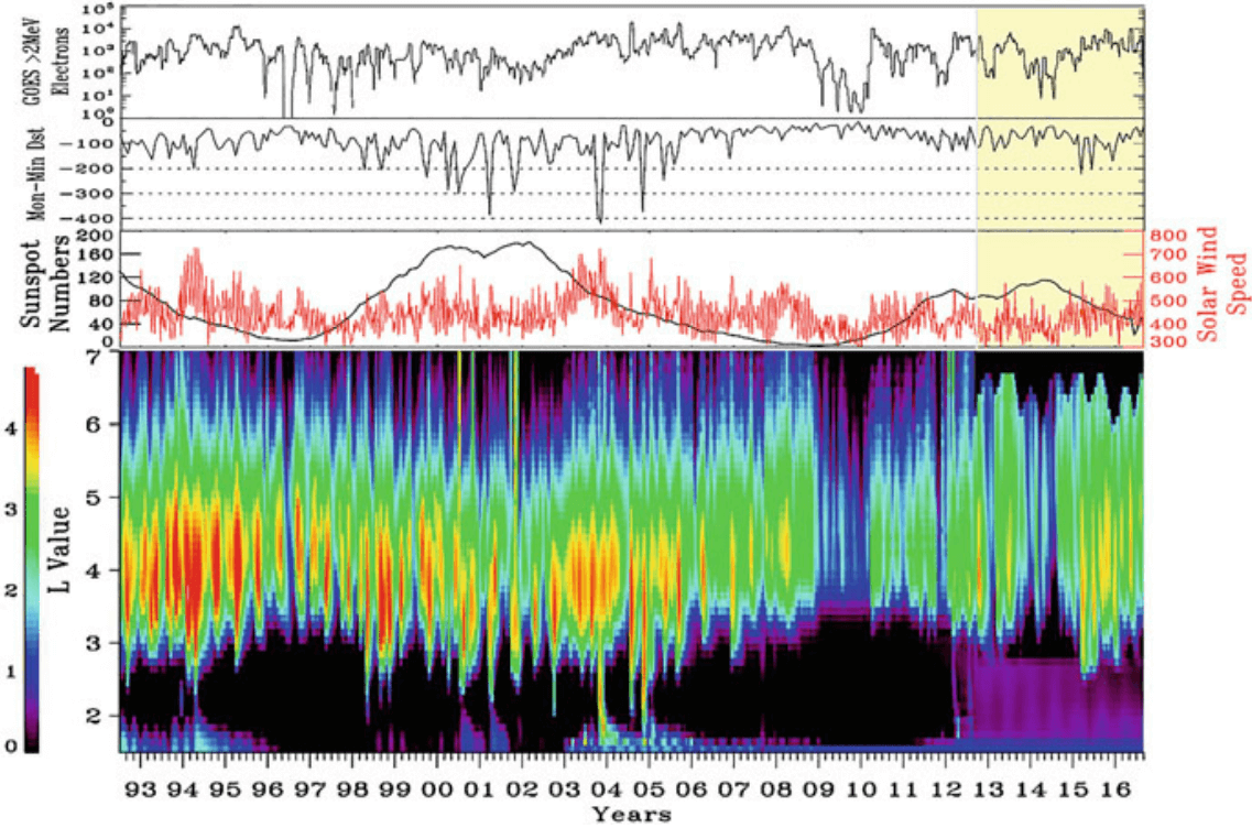
As illustrated in Figure 22.9, the storms are periods of most dynamic evolution of radiation belts. They often, but not always, commence with a significant positive deviation in the horizontal component of the magnetic field (H) measured on the ground (Figure 22.10), called storm sudden commencement (SSC). An SSC is a signature of an ICME-driven shock and the associated pressure pulse arriving at the Earth’s magnetopause. SSCs are also observed during pressure pulses related to SIRs or to ICMEs that are not sufficiently fast to drive a shock in the solar wind but still disturb and pile-up the solar wind ahead of them. If the solar wind parameters are known, the pressure effect can be removed from the Dst index as given by Equation 22.6.

Figure 22.9: Outer radiation belt response to solar and magnetospheric activity from the SAMPEX satellite and Van Allen Probes observations over a period of more than two solar cycles. The uppermost panel shows 27-day window-averaged relativistic (>2 MeV) electron fluxes at geostationary orbit, the second panel the monthly minimum of the Dst index, and the third panel the yearly window-averaged sunspot number (black) and weekly window-averaged solar wind speed (red). The spectrogram in the lowest panel is a composite of 27-day window-averaged SAMPEX observations of relativistic (∼2 MeV) electron fluxes until September 2012 and Van Allen Probes REPT observations of (∼2.1 MeV) electron fluxes after 5 September 2012. The shift from SAMPEX to Van Allen Probes is visible in the change of sensitivity to particle flux in the slot region (Li et al. 2017)

Storms in the magnetosphere can also be driven by low-speed ICMEs and SIRs without a significant pressure pulse. SIR-driven storms occur if the field fluctuations have sufficiently long periods of strong enough southward magnetic field to sustain global convention electric field to enhance the ring current. Thus there are storms without a clear SSC signature in the Dst index. On the other hand, a shock wave hitting the magnetopause is not always followed by a geomagnetic storm, in particular, if the IMF points dominantly toward the north during the following solar wind structure. In such cases the positive deviation in the magnetograms is called a sudden impulse (SI), after which the Dst index returns close to its background level with small temporal variations only. If the dynamic pressure remains at enhanced level, Dst can maintain positive deviation for some period.

After the SSC an initial phase of the storm begins. It is characterized by a positive deviation of Dst, typically a few tens of nT. The initial phase is caused by a combination of predominantly northward IMF and high dynamic pressure. The phase can have very different durations depending on the type and structure of the solar wind driver. It can be very brief if the storm is driven by an ICME with a southward magnetic field following immediately a sheath with predominantly southward magnetic field. In such a case the storm main phase, which is a period characterized by a rapid decrease of the H component of the equatorial magnetic field, starts as soon as the energy transfer into the magnetosphere has become strong enough. If the sheath has a predominantly northward IMF, the main phase will not begin until a southward field of the ejecta enhances reconnection on the dayside magnetopause.

If there is no southward IMF either in the sheath or in the ICME, no regular global storm is expected to take place. However, pressure pulses/shocks followed by northward IMF can cause significant consequences to the radiation belt environment, as they can shake and compress the magnetosphere strongly and trigger a sequence of substorms (Section 22.3.3).

Figure 22.10: The horizontal component (H) of the magnetic field measured at four low-latitude stations during a magnetic storm on 15 May 1997. An ICME-driven solar wind shock hit the magnetosphere on 15 May at about 02 UT causing the storm sudden commencement which is indicated by a sudden positive jump of the H component at all stations (thick blue line). The main phase of the storm started after 06 UT as indicated by the strong negative deviation in the H component. The solid vertical lines give the UT midnight and the tick-marks on the horizontal axis are given for each 3 h.

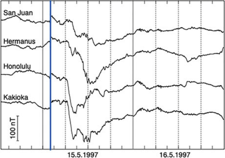
During the storm main phase, the enhanced energy input from the solar wind leads to energization and increase of the number of ring current carriers in the inner magnetosphere, as the enhanced magnetospheric convection transports an increasing amount of charged particles from the tail to the ring current region. Here substorms, discussed below, have important contribution, as they inject fresh particles from the near-Earth tail. The ring current enhancement is typically asymmetric because not all current carrying ions are on closed drift paths but a significant fraction of them passes the Earth on the evening side and continue toward the dayside magnetopause. This is illustrated in Figure 22.10 where the Honolulu and Kakioka magnetometers show the steepest main phase development when these stations were in the dusk side of the globe.

When energy input from the solar wind ceases, the energetic ring current ions are lost faster than fresh ones are supplemented from the tail. The Dst index starts to return toward the background level. This phase is called the recovery phase. It is usually much longer than the main phase, because the dominating loss processes of the ring current carriers: charge exchange with the low-energy neutral atoms of the Earth’s exosphere, wave–particle interactions, and Coulomb collisions, are slower than the rapid increase of the current during the main phase. As ICMEs last typically 1 day, storms driven by ICMEs trailed by a slow wind tend to have relatively short recovery phases, whereas storms driven by SIRs and ICMEs followed by a fast stream can have much longer recovery phases. This is because Alfvénic fluctuations, i.e., large-amplitude MHD Alfvén waves, in fast streams interacting with the magnetospheric boundary lead to triggering substorms, which inject particles to the inner magnetosphere. This can keep the ring current populated with fresh particles up to or longer than a week. The ring current development can also be more complex, often resulting in multi-step enhancement of Dst or events where Dst does not recover to quiet-time level between relatively closely-spaced intensifications. This typically occurs when both sheath and ICME ejecta carry southward field or when the Earth is impacted by multiple interacting ICMEs.

22.3.3 Substorms

Magnetospheric substorm is a transient solar-wind energy storage and release process within the magnetotail. It can inject fresh particles in the energy range from tens to a few hundred keV from the tail plasma sheet into the inner magnetosphere. After being injected to the quasi-dipolar magnetosphere, charged particles start to drift around the Earth, contributing to the ring current and radiation belt populations. The injections have a twofold role: They provide particles to be accelerated to high energies. Simultaneously the injected electrons and protons drive waves that can lead to both acceleration and loss of radiation belt electrons and ring current carriers.

Magnetospheric substorms result from piling of tail lobe magnetic flux in the near-to-mid-tail region during enhanced convection. The details of the substorm cycle are still debated after more than half a century of research. Observationally it is clear that substorms encompass global configurational changes in the magnetosphere, namely the stretching of the near-Earth nightside magnetic field and related thinning of the plasma sheet during the flux pile-up (substorm growth phase), followed by a relatively rapid return of the near-Earth field toward a dipolar shape (expansion phase), and a slower return to a quiet-time stretched configuration associated with thickening of the plasma sheet (recovery phase). A substorm cycle typically lasts 2–3 h. The strongest activity occurs following the onset of the expansion phase: The cross-tail current in the near-Earth tail disrupts and couples to the polar region ionospheric currents through magnetic field-aligned currents forming the so-called substorm current wedge. This leads to intense precipitation of magnetospheric particles causing the most fascinating auroral displays. During geomagnetic storms the substorm cycle may not be equally well-defined. For example, a new growth phase may begin and the onset of the next expansion may follow soon after the previous expansion phase.

A widely used, though not the only, description of the substorm cycle is the so-called near-Earth neutral line model (NENL model, for a review, see Baker et al. (1996)). In the model the current sheet is pinched off by a new magnetic reconnection neutral line once enough flux has piled up in the tail. The new neutral line forms somewhere at distances of 8–30 \(R_E\) from the Earth, which is much closer to the Earth than the far-tail neutral line of the Dungey cycle. Earthward of the neutral line plasma is pushed rapidly toward the Earth. Tailward of the neutral line plasma flows tailward, and together with the far-tail neutral line, a tailward moving structure called plasmoid forms. Sometimes recurrent substorm onsets can create a chain of plasmoids. While it is common to illustrate the plasmoid formation using two-dimensional cartoons in the noon–midnight meridional plane, the three-dimensional evolution of the substorm process in the magnetotail is far more complex. In reality a plasmoid is a magnetic flux rope whose two-dimensional cut looks like a closed loop of magnetic field around a magnetic null point.

As pointed out in Section 22.3.2, the plasma flow in the central plasma sheet is not quite smooth and a significant fraction of energy and mass transport takes place as bursty bulk flows (BBFs). The BBFs are thought to be associated with localized reconnection events in the plasma sheet roughly at the same distances from the Earth as the reconnection line of the NENL model. They create small flux tubes called dipolarizing flux bundles (DFBs). The name derives from their enhanced northward magnetic field component \(B_z\) corresponding to a more dipole-like state of the geomagnetic field compared to a more stretched configuration. Once created, DFBs surge toward the Earth due to the force caused by magnetic curvature tension in the fluid picture. They are preceded by sharp increases of \(B_z\) called dipolarization fronts. DFBs are also associated with large azimuthal electric fields, up to several \(\mathrm{mV}\,\mathrm{m}^{-1}\), which are capable of accelerating charged particles to high energies. Whether the braking of the bursty bulk flows and coalescence of dipolarization fronts closer to the Earth cause the formation of the substorm current wedge, or not, is a controversial issue.

The NENL model has been challenged by the common observation that the auroral substorm activation starts at the most equatorward arc and expands thereafter poleward. Another model proposed is the current disruption (CD) model, which is built upon plasma instabilities. In the CD model, a three-dimensional plasma instability grows first near the Earth in the transition region between the stretched tail and the dipolar inner magnetosphere. This instability drives steepening waves, leading to current disruption as the tail current cannot be sustained within a strongly oscillating geometry. The current disruption then launches tailward-propagating waves, which later trigger reconnection, plasmoid and fast flows. An easy way to think about these two models is that NENL is “outside-in”, while CD is “inside-out”. As both the current disruption and the plasma release from reconnection occur in only a few minutes, albeit roughly 100,000 km apart, it is challenging to uncover why and how the current disruption and plasmoid ejection take place. Setting aside the debate between competing explanations, what is essential is that the substorm expansions dipolarize the tail magnetic field configuration having been stretched during the growth phase and inject fresh particles into the inner magnetosphere. The particle injections can be observed as dispersionless, meaning that injected particles arrive to the observing spacecraft simultaneously at all energies, or dispersive when particles of higher energies arrive before those of lower energies. Because the dispersion arises from energy-dependent gradient and curvature drifts of the particles, a dispersionless injection suggests that the acceleration occurs relatively close to the observing spacecraft, whereas dispersive arrival indicates acceleration further away from the observation when the particle distribution has had time to develop dispersion due to energy-dependent drift motion.

Dispersionless substorm injections are typically observed close to the midnight sector at geostationary orbit (6.6 \(R_E\)) and beyond, but have been found all the way down to about 4 \(R_E\) (Friedel, Korth, and Kremser 1996). The injection sites move earthward as the substorm progresses and are also controlled by geomagnetic activity, although the extent of the dispersionless region is unclear, both in local time and radial directions. Neither have the details of acceleration of the injected particles been fully resolved. It has been suggested to be related both to betatron and Fermi acceleration associated with earthward moving dipolarization fronts. Another important aspect of dipolarization fronts for radiation belts is their braking close to Earth, which can launch magnetosonic waves that can effectively interact with radiation belt electrons.

22.4 ULF Waves

Ultra-low frequency (ULF) waves refer to waves within frequency range [0.001, 10] Hz. The name does not tell us anything about their physical origin, but simply observational fact. At Earth’s magnetosphere, this frequency range overlaps largely with the MHD waves. This is the reason why early pioneers in space physics relied on MHD theory for large spatial and temporal scales to explain the physics behind these waves, albeit some deviations and deficiencies which require more refined models such as the Vlasov description. ULF waves permeate the near-Earth plasma environment and play an important role in its dynamics, for example in transferring energy from the solar wind to the magnetosphere or accelerating electrons in the Earth’s radiation belts.

ULF waves were originally called micropulsations or magnetic pulsations since they were first observed by ground magnetometers. ULF pulsations are classified into two types: pulsations continuous (Pc) and pulsations irregular (Pi) with several subclasses (Pc1–5 and Pi1–2) according to their frequencies and durations. The division is based on their physical and morphological properties, and the boundaries are not strict.

Notation	Period Range [s]	Property
Pc1	0.2 - 5	EMIC
Pc2	5 - 10	EMIC, Mirror
Pc3	10 - 45	Foreshock, FLR, Mirror
Pc4	45 - 150	FLR
Pc5	150 - 600	SW, FLR
Pi1	1 - 40
Pi2	40 - 150

With respect to polarization, field line resonant ULF waves can be categorized into three modes: compressional (\(\Delta B_\parallel,\, \Delta E_\phi\))⁴, poloidal (\(\Delta B_r,\, \Delta E_\phi\)), and toroidal (\(\Delta B_\phi,\, \Delta E_r\)). Here, \(B_r\) (\(E_r\)), \(B_\parallel\), and \(B_\phi\) (\(E_\phi\)) are the radial, parallel (or compressional), and azimuthal components in the local magnetic field system, respectively. Referring to the basic MHD theory, the compressional modes are fast modes, whereas the poloidal and toriodal modes are Alfvén modes. The perturbed EM fields are related by \(\mathbf{B}_1 = \frac{\mathbf{k}}{\omega} \times \mathbf{E}_1\). Think of a closed field line near the equatorial plane inside the magnetosphere: if the wave vector \(\mathbf{k}\) is along the field line, i.e. \(\mathbf{k} = (0,0,k_z)\), then there will be two cases for the EM field: poloidal where \(\mathbf{E}_1\) in \(\hat{\phi}\), \(\mathbf{B}_1\) in \(\hat{r}\) and toroidal where \(\mathbf{E}_1\) in \(\hat{r}\), \(\mathbf{B}_1\) in \(\hat{\phi}\). If the wave vector \(\mathbf{k}\) is perpendicular to the field line, i.e. \(\mathbf{k} = (k_x, 0, 0)\), since there is no \(E_\parallel\) in MHD, we only have one option \(\mathbf{E}_1\) in \(\hat{\phi}\) and \(\mathbf{B}_1\) in \(\hat{z}\). A phase shift is allowed, and actually in real observations (e.g. THEMIS) it is rare that you can find B and E changing in-phase. These classifications are summarised in Table 16.1.

22.4.1 Pc1 & Pc2

• Usually observed in the noon-afternoon MLT sector, easily detectable when following sudden impulses (SI) produced by sudden changes in the pressure of the solar wind plasma.
• A sudden compression of the magnetosphere by increased solar wind pressure causes maximum distortion of the quiet magnetospheric plasma near noon at high latitudes. It is on the fieldlines which thread this disturbed plasma that one is most likely to witness ULF emissions.
• Conversely, as suggested by Hirasawa (1981) sudden rarefactions of the magnetosphere would be expected to quench ULF wave growth by reducing the anisotropy and \(\beta\) of the plasma. (INTERESTING ONE, SHOULD CHECK AT SOMETIME!)
• Delay of 1-3 mins between the occurance of SI and the onset of the ULF emission (ground-based magnetometers)[^growth_rate]
• Drive the trapped proton radiation, greatly enhanced eV energy range protons along the B field, and energization of keV range protons caused by betatron acceleration (Arnoldy et al. 2005).

At Earth, Electromagnetic ion cyclotron (EMIC) waves are typically observed in Pc1 and Pc2 range. In the outer radiation belt, the frequency typically ranges between 0.1 to 5 Hz. The preferential region of occurrence of EMIC waves is known to be the afternoon magnetic local time (MLT) sector from ∼12:00 to ∼18:00 MLT in the region near the plasmapause and the plasmaspheric plume.

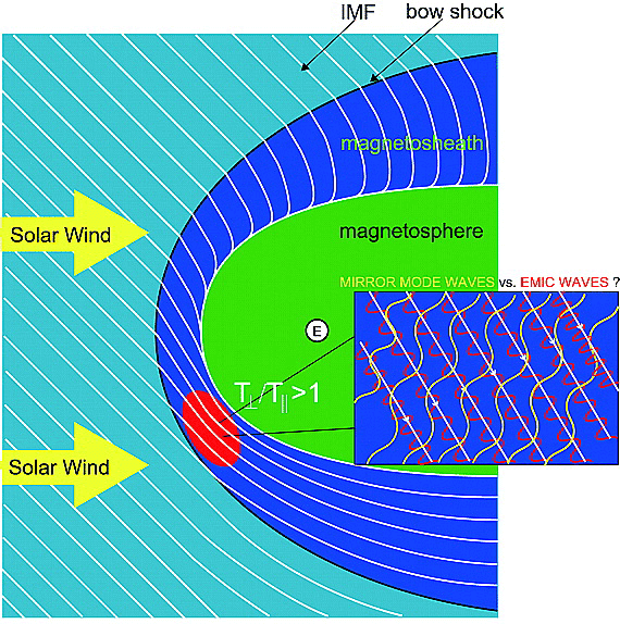
EMIC waves are normally excited by a temperature anisotropic (\(T_\perp > T_\parallel\)) distribution of hot (\(\sim 1-100\,\mathrm{keV}\)) ions. They are preferentially generated in regions where hot anisotropic ions and cold dense plasma populations spatially overlap (Figure 22.11).

Figure 22.11: Schematic sketch of chorus/EMIC wave excitation regions, denoted by dots, on the noon-midnight meridian plane.

The excited EMIC waves can result in the energization and loss of magnetospheric particles. Through resonant wave-particle interactions, EMIC waves are able to accelerate cold ions into the thermal (\(\sim 1\,\mathrm{eV} - 1\,\mathrm{keV}\)) energy range in the direction perpendicular to the ambient magnetic field, and cause the pitch angle scattering loss of hot ions in the ring current. Particularly, EMIC waves can also resonantly interact with relativistic electrons and result in pitch angle scattering of the electrons.

Newly excited EMIC waves are often transverse and left-hand polarized, consistent with the direction of ion gyration in the magnetic field (well, no surprise). After being generated, EMIC waves can be guided along the magnetic field lines and propagate from the source region to other magnetic latitudes. Spacecraft measurements have shown that EMIC wave propagation is almost exclusively away from the equator at latitudes greater than about \(11^\circ\), with minimal reflection at the ionosphere.

Some waves may even experience a polarization reversal where the wave frequency \(f\) is equal to the crossover frequency \(f_{co}\) during their higher-latitude propagation and then be reflected where \(f\) equals the bi-ion hybrid frequency \(f_{bi}\) at an even higher latitude. As a result, their polarization is crossed over from a left-hand to a right-hand or linear mode. These waves could undergo multiple equatorial crossings along magnetic flux tubes without a large radial or azimuthal drift. Because of their successive passes through the equatorial wave growth region, the waves are expected to be drastically amplified by continuing to obtain energy from the energetic protons. Nevertheless, Horne and Thorne argued that in the absence of density gradients, significant wave amplifications can only occur on the first equatorial pass because wave normal angles become large after the initial pass; wave damping by thermal heavy ions also makes it impossible for the same EMIC wave packet to bounce through its source region multiple times.

Mirror Instability & Ion Cyclotron Instability

Already, early observations in the 1970s have shown that the magnetosheath is populated by intense magnetic field fluctuations at time sclaes from 1 s to 10 s of seconds. Later research based primarily on data from ISEE and AMPTE satellites has shown that the mirror mode waves (Section 14.2) and kinetic Alfvén ion cyclotron (AIC) waves (i.e. EMIC waves) constitute a large majority of magnetosheath ULF waves:

1. AIC/EMIC are found predominantly near the bow shock and in the plasma depletion layer⁵ (Song, Russell, and Gary 1994; Hubert et al. 1998).
2. Mirror mode waves dominate in the central and downstream magnetosheath but can occur immediately downstream of quasi-perpendicular shocks too. (Hubert et al. 1989)
3. ULF waves are generally stronger in the dayside magnetosheath.
4. More frequency EMIC wave occurrence during quasi-parallel shocks.

The ion cyclotron instability responsible for the generation of AIC waves often grows under the same conditions as the mirror instability and in the linear approximation should dominate in lower \(\beta\) plasmas. The mirror instability, on the other hand, should dominate in high ion \(\beta\) plasmas (Lacombe and Belmont 1995). Since the initial confirmation of the existence of mirror modes in the Earth’s magnetosheath, they have been observed throughout the heliosphere. A long-standing puzzle in space plasmas is the fact that mirror modes are often the dominant coherent magnetic structures even for low \(\beta\) plasmas.

Figure 22.12: Mirror mode waves vs. EMIC waves in the magnetosphere.

People tried to find an answer to this puzzle. A bunch of studies in late 1980s and early 1990s (e.g. [Gary+]) argued that the presence of \(\text{He}^{++}\) tends to increase the EMIC threshold while the mirror mode growth is less affected by the presence of \(\text{He}^{++}\) ions. Yoshiharu Omura and his student Shoji presented another possibility in 2009 with hybrid PIC simulations that even though EMIC modes have higher linear growth rate, they saturates an an earlier stage than the mirror modes, especially in higher dimensions (by comparing 2D and 3D results), so that mirror mode waves can gain more free energy from temperature anisotropy.

22.4.2 Pc3 & Pc4

As already noted above, in the beginning when people proposed the ULF wave Pc divisions, many underlying physics are still unclear. The boundaries are chosen based on the observation data back then and does not necessarily contain any physical meaning.

ULF waves in the Pc3 range, with periods between 10-45 s, are a common feature of the dayside magnetosphere, where they are frequently observed both by spacecraft and ground-based observatories. They are thought to originate from the ion foreshock, extending upstream of the Earth’s quasi-parallel bow shock (the angle between IMF and shock normal \(\theta_{Bn}\le 45^\circ\)). There, ULF waves in the Pc3 frequency range are produced by ion beam instabilities, due to the interaction of shock-reflected suprathermal ions with the incoming solar wind.

For the foreshock-related Pc3/4 waves, we have the following picture. After foreshock waves are generated, they propagate through the magnetosheath (with very few observations) and reach the magnetopause. They enter the dayside magnetopause and travel antisunward into the magnetosphere as compressional Pc3 fluctuations, transporting the wave energy towards the nightside. In the inner magnetosphere, they may couple to Alfvénic field line resonances (FLRs), where their frequency matches the eigenmodes of the Earth’s magnetic field lines. Pc3 FLRs was observed at low latitudes and Pc4 at midlatitudes [Yumoto+, 1985]. The amplitude of the compressional mode decays when moving further into the magnetosphere, yet they can sometimes be observed all the way to the midnight sector. Compressional Pc3 wave power associated with transmitted foreshock waves is confined near the equator. Statistical study also shows that equatorial Pc3 wave power is stronger in the prenoon or noon sector (under various geomagnetic activity levels), consistent with the foreshock extending upstream of the dawn flank bow shock for a Parker-spiral IMF orientation. However, contrary to Pc5 pulsations (150-600 s), Pc3 wave activity does not show a clear correlation with the level of geomagnetic disturbances.

Also, note that not all Pc3 waves are related to foreshock waves, thus we may have different survey results about the distribution of Pc3 waves. This hints the fact that we are far from understanding the whole physical mechanism of wave generation.

There are several mechanisms by which Pc3-4 ULF waves may propagate to high latitudes:

• Harmonics of fundamental mode Pc5 resonances. Such harmonics would be expected to exhibit the same form of amplitude and phase properties that characterize FLRs and should occur at the same time as the fundamental.
• Cavity modes (Chapter 16).
• Fast mode waves propagate without mode conversion through the magnetosphere directly to the ionosphere. Such waves are subject to refraction and diffraction on their passage through the magnetosphere and may be directed to high latitudes via Fermat’s Principle (???).
• Transistor model that invokes beams of precipitating electrons [Engebretson+ 1991] (???). The transistor model requires no wave mode coupling or wave propagation across field lines, rather the modulated precipitation of electrons in response to pressure fluctuations in the magnetosheath. The latter are attributed to the upstream ion-cyclotron resonance mechanism. The modulated electron beams convey wave information from the outer magnetosphere region containing the parent population of trapped electrons, to the near-cusp ionosphere. The resultant periodic precipitation would modulate the ionospheric conductivity and hence ionospheric currents equatorward of the cusp. Overhead field lines could then be excited by these modulated currents equatorward of the cusp, with the same frequency as the modulated electrons. Engebretson likened this behavior to that of a transistor, where a small base current modulates a larger flow from collector to emitter. These ULF waves are characterized by noise-like appearance and low coherence lengths.

22.4.3 Pc5

We learned from ground, ionospheric, and space observations about the existence of only one or at least a few resonant field line vibrations (i.e. eigenoscillations) in the Pc5 range in the magnetosphere. As the Alfvén velocity is varying in the radial direction and as most sources of magnetospheric hydromagnetic waves are broadband sources, the resonance condition can be matched at an infinite number of geomagnetic field lines. Thus, every field line should be in resonance for a broad enough energy source. Therefore the observational fact of “magic” frequencies requires a magnetospheric frequency selection rule. (Kivelson and Southwood 1985) suggested that perturbations due to a broadband source at, e.g., the magnetopause first couple to the discrete eigenoscillations of global compressional eigenmodes. These narrow band compressional modes then couple to Alfvénic perturbations due to the field line resonance mechanism. The global modes thus select the frequency components participating in the resonant coupling. An alternative way of selection has been proposed by [Fujita+, 1996], who demonstrated that the K-H instability at the surface of a non-uniform magnetospheric plasma introduces dispersive properties of the unstable waves, which then gives rise to a narrower source spectrum. Thus, the field line resonance concept as outlined in Chapter 16 is able to explain the major features of observed resonant ULF pulsations in the terrestrial magnetosphere.

22.4.4 Sinks

According to (D. Southwood and Hughes 1983), possible sinks of ULF wave energy include at least three mechanisms:

• damping through ionospheric Joule heating,
• generalized Landau damping, and
• mode coupling.

By comparing the effects of Landau damping, Joule heating, and waveguide propagation, later researchers found from case studies that Joule heating and magnetospheric waveguide propagation are insufficient to account for the observed decay rate of ULF wave energy; Landau damping of the wave due to drift-bounce resonance with energetic ions was probably stronger, and more efficient when heavy ions such as \(O^+\) are present.

22.4.5 Interaction with Energetic Particles

22.4.5.1 Resonance

A widely used theory of energetic particle modulation by ULF transverse waves was developed by (D. J. Southwood and Kivelson 1981, 1981). In their theory, particles experience the wave-carried electric field during their drift-bounce motion and their energy is accordingly changed. The drift-bounce resonance of energetic particles is determined from \[ \Omega - m\omega_d = N\omega_b \tag{22.7}\] where \(N\) is an integer (normally \(\pm 1, \pm 2\) or \(0\)), \(m\) represents the azimuthal mode number of the ULF wave, and \(\Omega,\omega_d\) and \(\omega_b\) are the wave frequency and particle drift and bouce frequencies, respectively. \(N=0\) is known as the drift resonance whereas \(N\neq 1\) is the drift-bounce resonance. Because of the known energy dependence of \(\omega_d\) and \(\omega_b\), the resonance energy can be calculated if the wave properties (\(\Omega\) and \(m\)) are known. Observations from MMS and Cluster can be found in the review paper by Zong, Rankin, and Zhou (2017).

For particles of charge \(q\) experiencing drift motion in a ULF wave, the kinetic energy \(W\) changes at the following rate: \[ \frac{\mathrm{d}W_\mathrm{A}}{\mathrm{d}t} = q \mathbf{E}\cdot\mathbf{v}_\mathrm{d} \tag{22.8}\] where subscript \(\mathrm{A}\) signifies an average over many gyration periods, \(\mathbf{E}\) is the wave associated electric field, and \(\mathbf{v}_\mathrm{d}\) is the magnetic gradient and curvature drift velocity. For an equatorially mirroring particle (vanishing curvature drift) in Earth’s magnetic dipole field, the drift velocity \(\mathbf{v}_\mathrm{d}\) can be approximated in the nonrelativistic limit by \[ \mathbf{v}_\mathrm{d} = -\frac{3L^2 W}{q B_\mathrm{E}R_\mathrm{E}}\hat{e}_\phi \tag{22.9}\] where \(\hat{e}_\phi\) is defined eastward, \(R_\mathrm{E}\) is Earth’s radius, \(L\) is the L-shell parameter (radial distance in \(R_\mathrm{E}\) of the equatorial crossing point a field line), and \(B_\mathrm{E}\) is the equatorial magnetic field on Earth’s surface. ULF waves propagate in the azimuthal direction with the wave-associated electric field given by \[ \mathbf{E} = E_\phi \exp\,i(m\phi-\omega t)\hat{e}_\phi \tag{22.10}\] where \(\phi\) is the magnetic longitude (increasing eastward), \(m\) is the azimuthal wave number, and \(\omega\) is the wave angular frequency. From (Equation 22.8, Equation 22.9, Equation 22.10) the average rate of change of the particle energy is thus given by the following equation: \[ \frac{\mathrm{d}W_\mathrm{A}}{\mathrm{d}t} = -\frac{3L^2 W}{B_\mathrm{E}R_\mathrm{E}}\cdot E_\phi \exp\,i(m\phi-\omega t) \tag{22.11}\] which should be integrated along the particle drift orbit to \(t=-\infty\) to achieve an energy gain \(\delta W_\mathrm{A}\) from waves. Here, the particle’s drift orbit is assumed to be unperturbed (despite the energy change of the particle from the waves) with the angular drift frequency \(\omega_\mathrm{d}\) given by \[ \omega_\mathrm{d} = \frac{\mathrm{d}\phi}{\mathrm{d}t} = -\frac{3L^2 W}{B_\mathrm{E}R_\mathrm{E}^2} \tag{22.12}\]

An integration of Equation 22.11 backward in time along the particle’s drift orbit Equation 22.12 leaves a result that depends on the initial condition assuming the amplitude of the sinusoidal waves remains constant. To circumvent this problem, Southwood and Kivelson (1981) assumed the wave angular frequency \(\omega\) is complex with a small, positive imaginary part \(\Im(\omega)\) that represents a gradually growing wave signal. This assumption enables the particle to see a sinusoid for a finite interaction time, which on integration of Equation 22.11 yields an averaged particle energy gain (???) \[ \delta W_\mathrm{A} = -i\cdot\frac{3L^2 W}{B_\mathrm{E}R_\mathrm{E}}\frac{E_\phi\exp\,i(m\phi-\omega t)}{\omega-m\omega_\mathrm{d}} \tag{22.13}\]

Drift resonance happens when the particle drifts at the same azimuthal speed as the wave phase velocity, which indicates that \(m\omega_\mathrm{d} = \Re(\omega)\) so that the denominator of Equation 22.13 becomes \(\Im(\omega)\times i\). This small imaginary term suggests that for resonant particles, \(\delta W_\mathrm{A}\) must oscillate at a large amplitude in antiphase with the wave electric field. For particles with lower or higher energies (smaller or larger \(\omega_\mathrm{d}\)) the denominator is dominated by its real part and the corresponding \(\delta W_\mathrm{A}\) oscillations have much smaller amplitudes and are \(\pm 90^\circ\) out-of-phase with the wave electric field. In other words the amplitude \(\delta W_\mathrm{A}\) of energy gain must shift in phase by \(180^\circ\) as the resonance is crossed from low energy to high energy.

An actual particle detector cannot measure \(\delta W_\mathrm{A}\) directly, thus Southwood and Kivelson (1981) discussed the associated variations of particle fluxes and phase space densities (PSDs) that theoretical results can be compared directly with observational data. By assuming a negligible gradient of pre-existing particle PSDs in the azimuthal direction, the wave-produced PSD variations, \(\delta f_\mathrm{A}\), can be written as \[ \delta f_\mathrm{A} = \delta W_\mathrm{A}\left[ \frac{L}{3W}\frac{\partial f(W,L)}{\partial L} - \frac{\partial f(W,L)}{\partial W} \right] \] which shows that \(\delta f_\mathrm{A}\) is proportional to \(\delta W_\mathrm{A}\) provided there is a pre-existing finite PSD gradient in energy and/or space. Here, the importance of spatial gradients in producing PSD oscillations is emphasized, which is caused by back-and-forth convection of particles as a response to the wave electric field. The PSD variations can be alternatively written as \[ \delta f_\mathrm{A} = -\delta W_\mathrm{A}\frac{\partial f(W,\mu)}{\partial W} = \delta W_\mathrm{A}\frac{L}{3W}\frac{\partial f(L,\mu)}{\partial L} \] where \(\mu\) is assumed to be constant for adiabatic behavior of particles interacting with ULF waves. The linear dependence of \(\delta f_\mathrm{A}\) on \(\delta W_\mathrm{A}\) suggests that the phase shift of particle PSDs across theresonant energy should also be \(180^\circ\). Such a phase shift is thus treated as a characteristic signature of ULF wave-particle drift resonance.

22.4.5.2 Particle trapping by compressional waves

The mirror force produced by the magnetic field-aligned component of compressional mode ULF waves can also modulate energetic particle fluxes. Observational evidence from Van Allen Probes can be found in the citations of Zong, Rankin, and Zhou (2017).

22.4.5.3 Fast acceleration of charged particles by ULF waves

The theory of drift-bounce resonance developed by Southwood and Kivelson (1981, 1981) is valid for axisymmetric magnetic fields. In this case, particles experience the wave electric field along their drift and bounce motion and suffer net energy gain or loss when the resonance condition Equation 22.7 is satisfied, usually for \(N=0,\pm 1, \pm 2\). Parallel electric fields are neglected as they are usually small in collisionless plasma⁶. The rate of energy change of a charged particle interacting with a ULF wave is expressed by \[ \frac{\mathrm{d}W}{\mathrm{d}t} = \mu\frac{\partial B_\parallel}{\partial t} + q\mathbf{E}\cdot\mathbf{v}_\mathrm{d} \] where \(\mathbf{E}, \mathbf{v}_\mathrm{d}\) and \(\mu\) denote the wave electric field, particle drift velocity, and magnetic moment, respectively. The first and second terms on the right-hand-side of the equation represent acceleration due to the wave magnetic and electric fields, respectively.

In an asymmetric compressed dipole field, a particle can resonant with low-m global toroidal waves when the wave frequency satisfies \(\omega=(m\pm 1)\omega_d\). For example, Elkington, Hudson, and Chan (1999) showed that in a magnetic topology with noon-midnight asymmetry electrons can gain energy from toroidal ULF waves; in other words, toroidal ULF waves can accelerate energetic particles in he radiation belt region under strong solar wind pressure. However, in the inner magnetosphere noon-midnight asymmetry becomes insignificant on low L-shells. Acceleration of energetic electrons by toroidal mode ULF waves may, therefore, be limited to the outer magnetosphere, while in the inner magnetosphere the poloidal mode is more likely responsible. However, in the dayside outer magnetosphere the poloidal electric field of fast mode wave may also accelerate energetic electrons.

22.4.6 EMIC Wave Events

(Usanova and Mann 2016)

EMIC waves are believed to be important for influencing the dynamics of energetic particles in the inner magnetosphere, especially in relation to ring current and radiation belt dynamics. In relation to the ring current, both the dynamical evolution of ion distributions along their drift paths and effects from the solar wind can result in EMIC wave generation from unstable ion distributions. EMIC waves often grow as a result of perpendicular temperature anisotropy, with the ion dynamics and energy and pitch angle distributions in the ring current being modified significantly by the growth of the EMIC instability. EMIC waves are also hypothesized to influence higher energy electrons in the Van Allen belts, through a Doppler-shifted cyclotron resonance, including stimulating potential scattering loss into the atmosphere.

The prevalence of dayside EMIC activity during intervals of enhanced solar wind dynamic pressure can be explained by three possible mechanisms, which can lead to the generation of anisotropic proton distributions.

22.4.6.1 Bursty EMIC wave events

Short-term magnetospheric compressions can increase the \(A=T_\perp/T_\parallel\) ratio through adiabatic heating and can generate EMIC wave bursts during periods within which the magnetic field strength is increasing (i.e. \(dB/dt>0\)). In a dipole field, the resulting anisotropy is generated if the magnetic field magnitude changes from the initial value \(B_0\) to the final value \(B\), \[ A = \left(\frac{B}{B_0}\right)^{1/3}(A_0 + 1) - 1 \] where \(A_0\) is the initial anisotropy (Olson and Lee 1983). I did not read carefully about the original paper, but I feel like this is related to Equation 14.22 and betatron acceleration.

22.4.6.2 Continuous EMIC waves events

Continuous EMIC waves events may be seen to last for several hours in ground-based magnetometer data, often occurring during intervals while the magnetosphere remains compressed in response to a continuous period of enhanced solar wind dynamic pressure. There are two proposed physical mechanisms which may result in the generation of this type of long-lasting and continuous EMIC wave event.

Figure 22.13: Schematic illustrating mechanisms for continuous EMIC wave event: (a) drift shell splitting and (b) Shabansky orbit [adapted from Usanova 2010b]. (a) Drift path of \(30^\circ\) (orange) and \(90^\circ\) (red) pitch angle protons from the nightside to the dayside magnetosphere; a schematic of the descreasing logarithm of proton flux (green) as a function of radial distance from the Earth is also shown. (b) Trajectory of a proton whose bounce trajectory changes from trapping between mirror points spanning the equatorial plane to trapping between two off-equatorial minimum B regions, resulting in trajectories which do not cross the equatorial plane in the dayside magnetosphere (also known as Shabansky orbits).

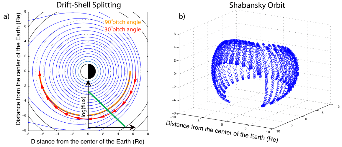
• Drift-Shell Splitting

Particles with different pitch-angles follow different drift paths, such that particles from different spatial locations can be brought together to create an unstable distribution. While in a symmetric dipolar magnetic field all particles drift around the Earth at the same (initial) equatorial distance, in a compressed magnetic field particles with near \(90^\circ\) pitch angles follow lines of constant magnetic field (conserving magnetic moment), and particles with smaller pitch-angles move along more circular orbits. This is known as drift-shell splitting, which is illustrated by the schematic in Figure 22.13 a.

Figure 22.13 a shows example drift paths of particles with pitch angles of \(30^\circ\) and \(90^\circ\) as they drift from the nightside to the dayside in the magnetosphere. The drift paths of these two particles intersect at the dayside subsolar magnetosphere, while the initial starting point of their trajectories was located in the nightside magnetosphere in two different locations: for a \(30^\circ\) pitch angle particle further away from the Earth and for a \(90^\circ\) pitch angle particle closer to the Earth. In a situation where the flux of particles decreases with radial distance from the Earth as shown in Figure 22.13 a the \(90^\circ\) pitch-angle particles drift closer to the Earth, as compared to smaller pitch-angle particles, will have a larger flux. This leads to an enhancement of the perpendicular temperature with respect to the parallel temperature and makes the distribution temperature anisotropic (with \(T_\perp > T_\parallel\)), and thereby potentially unstable to EMIC waves. The drift trajectory splitting is more prominent for particles at higher L-shells and for higher degrees of compression. Therefore, for the inner magnetosphere this effect may be important only during intervals of highly increased solar wind dynamic pressure.

• Shabansky Orbit

The outer L-shells of the compressed dayside magnetosphere can have two off-equatorial minima in magnetic field strength, which are more pronounced during strong compressions, and can be regarded as a compression-related feature of the reconfigured dayside magnetospheric magnetic field. In such a field topology, particles with \(90^\circ\) pitch angles continue to drift through the equator, but particles with lower pitch angles can mirror at high latitudes without passing through the equator, executing so-called “Shabansky” orbits [Shabansky, 1971]. As particles reach the \(\partial B/\partial s < 0\) region near the dayside magnetopause, where \(S\) is distance along the magnetic field, they escape off-equator and execute repeated bounces and are trapped at mid-latitudes. This is demonstrated in Figure 22.13 b which shows the full trajectory of a proton drifting from the nightside to the dayside magnetosphere. These so-called Shabansky regions can lead to the formation of enhanced temperature anisotropy in two different locations: in the equatorial plane, where there is the absence of the lower pitch angle particles; and second, in the trapped off-equatorial regions where particles’ pitch angle undergoes a net shift towards a higher pitch angle. (???) As a result, the ion perpendicular temperature increases relative to the parallel temperature, with the resulting temperature anisotropy potentially giving rise to the growth of EMIC waves, especially in the off- equatorial regions. Similar to drift shell splitting, when magnetosphere is strongly compressed by the solar wind the regions supporting Shabansky orbits may move further inward, reaching locations inside geosynchronous orbit, to become an important source of dayside temperature anisotropy in the inner magnetosphere.

22.5 Bow Shock

Bow shock is the shock (Chapter 21) resulted from the interaction of supersonic, super-Alfvénic solar wind with the magnetosphere of an astrophysical object.

22.5.1 Foreshock

The word “foreshock” is borrowed from geophysics for an earthquake that occurs before a larger seismic event (the “mainshock”) and is related to it in both time and space. In space physics, foreshock is the region upstream from the bow shock that is magnetically connected to the bow shock and contains both solar wind plasma and also charged particles backstreaming from the bow shock. It is typically associated with quasi-parallel shocks, as it is much easier for charged particles to move freely along the normal direction of the shock if it is aligned with \(\mathbf{B}\). If their speed relative to the ambient plasma is fast enough, plasma shocks without Coulomb collisions cannot dissipate all the incoming plasmas; some of them have to “return”. The counter-streaming between the foreshock plasma and the incoming plasma is very unstable and thus excites many types of waves.

Figure 22.14: Foreshock configuration showing incident solar wind magnetic field (blue lines), impinging on the bow shock (green curved line), producing backstreaming ions (yellow dots), leaked magnetosheath ions (red dots), and upstream waves (wavy blue lines). The ion foreshock boundary is shown as the red line (Wilson III 2016). The foreshock boundary is the reflected ion trajectory tangent to the shock surface, taking into account the combination of a field-aligned motion and the solar wind convection electric field.

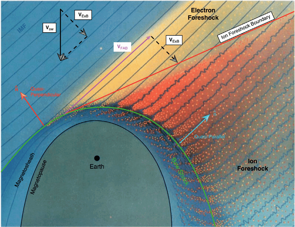
Figure 22.14 demonstrate the basic geometry of Earth’s foreshock. The slanted straight lines are the magnetic field embedded in the solar wind that is flowing downward in the figure and encounters the curved bow shock (green curve). The angle between the magnetic field and the normal direction at the shock is denoted as \(\theta_\mathrm{Bn}\). The portion of the bow shock where \(\theta_\mathrm{Bn} > 45^\circ\) (i.e., the region to the left of the Earth in the figure) is termed the “quasi-perpendicular shock”, while the region to the right, \(\theta_\mathrm{Bn} < 45^\circ\), is the “quasi-parallel shock” that extends all the way down to \(\theta_\mathrm{Bn} \sim 0^\circ\) - the “parallel shock”. At the shock near \(\theta_\mathrm{Bn} \sim 90^\circ\), some of the incoming solar wind electrons, which have small gyroradii, are reflected and propagate back upstream creating the region known as the “electron foreshock”. Some of the solar wind ions impinging on the bow shock near \(\theta_\mathrm{Bn} \sim 90^\circ\) are also reflected, but because they have larger gyroradii, quickly gyrate into the downstream. At somewhat smaller \(\theta_\mathrm{Bn}\), but still associated with the quasi-perpendicular bow shock, a fraction of the solar wind ions are also reflected and travel back upstream along the magnetic field as well as being convected in the solar wind (\(\mathbf{V}_{E\times B}\) in the figure) to form the quasi-perpendicular portion of the ion foreshock. Farther to the right of the ion foreshock boundary shown in Figure 22.14, ions originating at the shock at even smaller \(\theta_\mathrm{Bn}\), e.g., on the quasi-parallel portion of the shock, also propagate upstream (dots in the figure), generating larger amplitude waves in the magnetic field (blue wavy lines), to form the quasi-parallel portion of the ion foreshock. These backstreaming ions may have been from the solar wind and reflected at the shock or could have leaked out of the magnetosheath. This process extends deep in the foreshock to \(\theta_\mathrm{Bn} \sim 0^\circ\), where the shock normal is essentially parallel to the solar wind magnetic field.

The dominant wave mode in the ion foreshock is produced by the ion-ion beam right-hand instability and has a typical period around 30 s in Earth’s foreshock. Their exact period however varies significantly depending on the solar wind conditions, in particular the IMF strength, between 10 and 80 s. One easy way to think about this is by remembering the gyrofrequency \(\omega_c=qB/m\): the beam instabilities are associated with the cyclotron resonance, and the gyrofrequency is directly related to \(B\). Their wavelength is of the order of \(1\,\text{R}_\text{E}\) and they are left-hand polarized in the spacecraft frame. Their intrinsic polarization is however right-handed, indicative of a fast mode. The polarization reversal is due to the waves attempting to propagate sunward, while they are effectively carried earthward by the faster solar wind flow. The fast mode is also consistent with the observed positively correlated magnetic field strength and plasma density fluctuations.

The ion-ion right-hand resonant instability is driven by ion beams that are cold and fast, streaming back from the bow shock along the magnetic field, characteristically produced in the quasi-perpendicular portion of the foreshock. During the initial growth of the instability, the excited electromagnetic waves have group velocities close to the beam speed, so that the field energy propagates with the beam. The waves pitch-angle scatter the beam reducing the free energy.

Electromagnetic ion beam instabilities with somewhat different properties are also found deeper in the foreshock on magnetic field lines that connect to the nearly parallel portion of the bow shock. Here the ion beams are slower and hotter and instead of being generated by reflection at the shock, are more likely to result from heating and scattering of the cold beam ions, processes related to the unsteady nature of the parallel shock, or from magnetosheath ions that leaked out into the foreshock. Other types of ion beam instabilities arise elsewhere in space, e.g., in the plasma sheet boundary layer upstream of slow-mode shocks in the magnetotail and in the vicinity of comets.

From spacecraft missions ISEE, Cluster and MMS, we have found two main populations of backstreaming ions, termed reflected and diffuse. The reflected ions have a sharply peaked energy spectrum and relatively collimated flow coming from the bow shock along the interplanetary magnetic field with number densities \(\sim 1.5\%\) of the solar wind. In contrast, the diffuse ions have a much flatter energy spectrum and broad angular distributions, with lower density \(\sim 0.7\%\) of the solar wind. These two populations occur in separate regions of the foreshock, with reflected ions in the quasi-perpendicular portion and the diffuse ions in the more nearly parallel portion of the foreshock, suggesting different mechanisms of origin and acceleration. In between the reflected and diffuse ion populations, were intermediate ions that had a crescent shape in velocity space, which corresponds to the gyro-phase bunched ions and pitch-angle scattering by the generated waves. The reflected ions were so named, because backstreaming beams of ions were observed traveling upstream in a direction determined by the interplanetary magnetic field and the convection velocity (\(\mathbf{V}_{E\times B}\)), consistent with simple models of specular reflection at the bow shock.

Observations from ISEE also showed that there were usually weak waves occurring with reflected beam ions, while with diffuse ions large amplitude, compressive waves often occurred. Obliquely propagating waves were also observed, often in the form of steepened waves, termed shocklets. In addition, deeper in the foreshock Alfven waves were also generated in associated with the diffuse ions. The location in the foreshock where the low frequency waves begin to appear, is called ULF foreshock boundary, near the ion foreshock boundary. Another wave produced deep in the foreshock near the quasi-parallel bow shock is termed short large-amplitude magnetic structures (SLAMS).

The linear theory of beam instabilities in magnetized plasmas is developed by Peter Gary. He numerically solved the complete dispersion relation for both electrostatic and electromagnetic waves excited by various sorts of free energy: i.e., beams of electrons or ions, temperature anisotropies in either the background or beam species, etc.⁷ In (Gary, Gosling, and Forslund 1981), he showed how a weak (~1% density) beam initially produces a low level of waves with growth times > 25 s. Because the growth rate of the waves is small, the ion beam propagates a long distance upstream from the bow shock before the waves grow to large amplitude. But in the process of propagating upstream, the beam ions and the waves are convected deep into the quasi-parallel portion of the foreshock, where they are slowed. The beam ions loses parallel momentum as they are pitch-angle scattered by the waves, producing intermediate velocity distributions (kidney shaped). This loss of energy and momentum by the beam, and the waves, causes the solar wind to be deflected and slowed, as observed by Bame et al. (1980). Since the compressibility (i.e., the density fluctuations computed from linear theory) of oblique waves⁸ is significantly larger than for parallel propagation, oblique waves can grow and produce density fluctuations in agreement with observations.

In Gary et al. (1984), four linear electromagnetic ion instabilities are compared (Section 21.6.1). Numerical solutions of the linear dispersion relation are presented to show that for parallel propagation the righthand resonant instability has a lower instability threshold than the non-resonant instability unless the beam speed or beam density is sufficiently large. For hot ion beams a left-hand resonant instability is also excited, and if there is a large temperature anisotropy in the beam (\(T_{b,\perp} \gg T_{b,\parallel}\)), a left-hand ion cyclotron instability is also possible. Therefore, the deterministic factors for the driven instabilities would be

• beam density \(n_b\)
• beam velocity \(V_b\) (w.r.t. \(V_A\))
• beam temperature \(T_b\)
• beam pressure anisotropy

In Gary, Thomsen, and Fuselier (1986), linear theory of both the right-hand resonant and non-resonant instabilities driven by an energetic, cool ion beam is used to calculate the phase angle between the fluctuating velocity of the beam ions relative to the fluctuating magnetic field in order to determine whether gyrophase bunching of the beam ions is observable. Distinct gyrophase-bunched ions have been observed in the foreshock by ISEE. Peter’s linear calculations showed that for the non-resonant mode, the phase angle is \(\sim 0^\circ\), while for the resonant mode it is \(\sim 90^\circ\) for the most unstable wavenumber. Both observations and simulations support the right-hand resonant instability for generating the observable gyrophase bunching for the ion beam.

Despite all these achievements, a major problem remains — the observed ULF waves are primarily propagating oblique to the magnetic field, contrary to linear theory that says the parallel mode has the largest growth rate and thus in time will become the dominant mode. Measurements by Cluster (Eastwood et al. (2005)) indicate a mean angle of \(21^\circ\). An even more interesting suggestion is given later by Strumik et al. (2015). In their foreshock simulations they assume that the solar wind is essentially radial. They find that while parallel unstable modes dominate, oblique waves are also generated, and when properly averaged over phase space density, the “average” propagation direction is \(\sim 20^\circ\), consistent with Eastwood et al. (2005).⁹

22.5.2 Transmission of Waves

An interesting question arises about the transmission of fast waves through the bow shock into the downstream. A list of possible mechanisms are summarized in Figure 22.15. (Turc et al. 2022) argued that the earthward magnetosonic disturbances can then propagate to and disturb the magnetopause, whereas shock reformation and mode conversion play only minor roles.

Figure 22.15: Foreshock waves (purple wavy lines) are generated in the region upstream from the bow shock (left black curve) where the interplanetary magnetic field (IMF) lines (dashed lines) are quasi-parallel to the shock normal \(\hat{n}\) (shaded blue). Foreshock waves are convected towards the bow shock by the solar wind (red arrow) and transmit through the magnetosheath via mechanisms indicated in the white boxes along the bow shock: mode conversion, shock reformation, and modulation of shock compression. The transmitted waves propagate away from or towards Earth relative to the magnetosheath plasma (indicated by the wave vector \(\mathbf{k}\)).

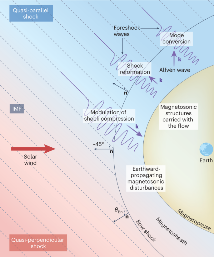
As usual in plasma physics, accompanying the ion foreshock we have electron foreshock at a much smaller scale.

The formation of ion/electron foreshocks requires counter-streaming of ions and electrons, respectively. Since there is only one velocity for each species in the electron/ion two-fluid equations, it is not possible to trigger this instability in a multi-moment model. Theoretically we may have an extremely simplified case where the ion counter-streaming is represented by two ion fluids, but there are very few studies on this topic. The minimum requirement may be gyrokinetics.

22.6 Magnetosheath

22.6.1 Jets

Magnetosheath jets are regions of enhanced dynamic pressure. Think of jets as raindrops in the magnetosheath falling on the magnetopause. They are widely associated with the quasi-parallel magnetosheath, suggesting that their origin is tied to the interactions between the foreshock and the bow shock.

The formation of magnetosheath jets may be related to both external and internal drivings.

• External
  • Solar wind pressure pulses
  • Rotational discontinuities
• Internal
  • Local ripples from foreshock turbulence could lead to the refraction and funneling of plasma.
  • Short large-amplitude magnetic structures (SLAMS), which are steepened foreshock fluctuations in a short time-scale but large spatial scale.

22.7 Magnetosphere

Figure 22.16: The magnetosphere with its current system.

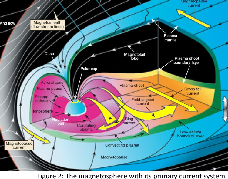
22.7.1 Magnetopause

The magnetopause is the abrupt boundary between a magnetosphere and the surrounding plasma. The collision frequency of particles in the plasma in the interplanetary medium is very low and the electrical conductivity is so high that it could be approximated to an infinite conductor. A magnetic field in a vacuum cannot penetrate a volume with infinite conductivity. Chapman and Bartels (1940) illustrated this concept by postulating a plate with infinite conductivity placed on the dayside of a planet’s dipole as shown in Figure 22.17. The field lines on the dayside are bent. At low latitudes, the magnetic field lines are pushed inward. At high latitudes, the magnetic field lines are pushed backwards and over the polar regions. The boundary between the region dominated by the planet’s magnetic field (i.e., the magnetosphere) and the plasma in the interplanetary medium is the magnetopause. Since the solar wind is continuously flowing outward, the magnetopause above, below and to the sides of the planet are swept backward into the geomagnetic tail as shown in the artist’s concept. The region (shown in pink in the schematic) which separates field lines from the planet which are pushed inward from those which are pushed backward over the poles is an area of weak magnetic field or day-side cusp. Solar wind particles can enter the planet’s magnetosphere through the cusp region. Because the solar wind exists at all times and not just times of solar flares, the magnetopause is a permanent feature of the space near any planet with a magnetic field.

Figure 22.17: Schematic representation of a planetary dipole magnetic field in a vacuum (right side) deformed by a region of plasma with infinite conductivity. The Sun is to the left. The configuration is equivalent to an image dipole (green arrow) being placed at twice the distance from the planetary dipole to the interaction boundary.

If one assumed that magnetopause was just a boundary between a magnetic field in a vacuum and a plasma with a weak magnetic field embedded in it, then the magnetopause would be defined by electrons and ions penetrating one gyroradius into the magnetic field domain. Since the gyro-motion of electrons and ions is in opposite directions, an electric current flows along the boundary.

22.7.1.1 Estimation of the standoff distance

The location of the magnetopause is determined by the pressure balance between the internal magnetic field and external solar wind. As a first order estimation of the standoff distance to the magnetopause, we neglect the internal magnetospheric thermal pressure and let the dynamic ram pressure from the solar wind being equal to the magnetic pressure from the Earth’s magnetic field:¹⁰ \[ \left( \rho v^2 \right)_\textrm{sw} \approx \left( \frac{4B(r)^2}{2\mu_0} \right)_\textrm{m} \] where \(\rho\) and \(v\) are the density and velocity of the solar wind, and \(B(r)\) is the magnetic field strength of the planet in SI units.

Since the dipole magnetic field strength varies with distance as \(1/r^3\) the magnetic field strength can be written as \(B(r)=B_0/r^3\), where \(B_0\) is the planet’s magnetic moment, expressed in \([\textrm{T}\cdot \textrm{m}^3]\). \[ \begin{aligned} \rho v^2 \approx \frac{2B_0^2}{r^6 \mu_0} \\ r \approx \left( \frac{2B_0^2}{\mu_0 \rho v^2} \right)^{1/6} \end{aligned} \]

The distance from Earth to the subsolar magnetopause varies over time due to solar activity, but typical distances range from \(6-15 R_{\oplus}\). Empirical models (e.g. (Shue et al. 1997)) using real-time solar wind data can provide a real-time estimate of the magnetopause location.

Table 22.2 summarizes the basic sizes of each planet in the solar system. Venus and Mars do not have a planetary magnetic field and do not have a magnetopause. The solar wind interacts with the planet’s atmosphere and a void is created behind the planet. In the case of the Earth’s moon and other bodies without a magnetic field or atmosphere, the body’s surface interacts with the solar wind and a void is created behind the body, often called wake. All planets may show the effect of inductance, depending on the conductivity of the ionosphere or ionosphere-like sphere. The interaction of IMF with a conductor induces current on the surface of the conductor and create an induced magnetic field which opposes the external field from penetrating into the conductor. This is a major contribution at Mars, a minor contribution at Mercury and Ganymede, and somehow being negligible at other large planets.

Table 22.2: Solar system magnetopauses

Planet	Magnetic Moment11	Standoff Distance12	Variance13
Mercury	0.0004	1.5	0
Venus	0	0	0
Earth	1	10	2
Mars	0	0	0
Jupiter	20000	42	25
Saturn	600	19	3
Uranus	50	25	0
Neptune	25	24	1.5

22.7.2 Transport of mass, momentum, and energy

Transport of mass, momentum, and energy at the magnetopause boundary drives much of the magnetospheric dynamics and is thus an important topic in magnetospheric physics. The amount of solar wind plasma and energy that enters the magnetosphere is regulated by the orientation of the interplanetary magnetic field (IMF): during southward IMFs, the major process is considered to be magnetic reconnections (Section 13.8), while during northward IMFs, the processes include cusp reconnection, plasma mixing/reconnection in Kelvin-Helmholtz vortices, and wave-particle diffusive processes in large-amplitude ULF waves at the magnetopause boundary (?sec-klr).

One of the more common spectral features at the magnetopause boundary is the sharp transition in wave polarization from compressional, e.g., because of foreshock waves of the quasi‐parallel bow shock, to transverse (Alfvén) waves from the magnetosheath to the boundary layers. Mode conversion from compressional to Alfvén modes through the magnetopause can efficiently transport and heat plasma across the boundary. Multipoint measurements have verified that the dispersion of the broadband waves is consistent with the kinetic Alfvén waves (KAWs) [Chaston+,2007, 2008]. KAWs also provide a natural explanation for the observed dawn‐dusk asymmetry in plasma entry during northward IMF because they result from mode conversion of compressional foreshock waves, which typically bathe the dawn flank for the typical Parker spiral configuration.

According to linear theory, when an MHD fast mode compressional wave propagates across in an inhomogeneous plasma, it is coupled with the shear Alfvén wave at the local Alfvén resonance \(\omega=k_\parallel V_A\), with \(\omega\) being the wave frequency. This process can be very efficient when the fast wave propagates into a region where there is a sharp increase in the Alfvén velocity such as at the magnetopause boundary where the magnetic field increases and density decreases. Typically, the Alfvén velocity across the magnetopause increases by a factor of 10 such that an entire decade (in frequency) of wave power can be captured and localized in the boundary layer leading to massive particle transport. In the MHD description, the coupling occurs where the frequency matches the continuous spectrum and the wave becomes singular corresponding to a pileup of compressional wave energy.

Singular behavior occurs at either the Alfvén resonance, \(\omega^2=k_\parallel^2 v_A^2\), or at the sound resonance, where the compressional wave couples with the Alfvén or sound wave that propagates only along the magnetic field. In higher frequency cases, the Alfvén resonance condition is modified because of the finite ion Larmor radius effects (Equation 16.27), where the Alfvén resonance singularity can be removed by including non‐MHD effects such as electron inertia or ion Larmor radius corrections in Equation 16.26. It can be shown that kinetic effects naturally arises from the two-fluid/kinetic theory, including the coupling to KAWs. For more equations, see Section 16.4.

At the resonance point, the fast wave solution is coupled to the KAW solution, and transversely polarized Alfvén waves are expected to be generated and radiate away from the mode conversion location. Because the group velocity of these waves is much smaller than the compressional wave, the amplitude of the transverse fluctuations is typically much larger than the amplitude of the compressional driver, consistent with magnetopause observations.

As been discussed in Chapter 16, when the azimuthal wave number \(m\), or \(k_y\) in the box model is zero, there should be no mode coupling. However, this is not true if the finite-frequency effect is considered (Section 16.4), as first noted by (1979).

22.7.3 Dungey Cycle

Dungey (1961) was the first to propose a cycle of magnetospheric convection driven by magnetic reconnection at the dayside magnetosphere. Magnetic field connected on the dayside of Earth is transported by the solar wind to the night side where it forms a long tail behind the Earth. This transfer of flux to the nightside forces the magnetosphere to undergo systematic changes in configuration that eventually lead to nightside magnetic reconnection, which returns flux to the dayside along the flanks of the magnetosphere via the different response modes.

22.7.4 Vasyliunas Cycle

The Jovian equivalent to the Dungey cycle of the Earth’s magnetosphere, where the centrifugal force plays a critical role in affecting the plasma convection.

22.7.5 Low-Latitude Boundary Layer

The Earth’s low-latitude boundary layer (LLBL) is the region where magnetosheath and magnetospheric plasmas are mixed along the magnetospheric side of the low-latitude magnetopause. It has been suggested that three processes — magnetic reconnection at high-latitudes, the Kelvin-Helmholtz instability, and Kinetic Alfvén waves — primarily contribute to the formation, all of which have been observed by in-situ satellites inside the LLBL. Recent studies further suggested that the couplings of these processes effectively enhance the formation rate.

Angelopoulos, Vassilis, Wo Baumjohann, CF Kennel, F Vo Coroniti, MG Kivelson, R Pellat, RJ Walker, H Lühr, and G Paschmann. 1992. “Bursty Bulk Flows in the Inner Central Plasma Sheet.” Journal of Geophysical Research: Space Physics 97 (A4): 4027–39. https://doi.org/10.1029/91JA02701.

Arnoldy, Roger L, MJ Engebretson, RE Denton, JL Posch, Marc R Lessard, NC Maynard, DM Ober, et al. 2005. “Pc 1 Waves and Associated Unstable Distributions of Magnetospheric Protons Observed During a Solar Wind Pressure Pulse.” Journal of Geophysical Research: Space Physics 110 (A7). https://doi.org/10.1029/2005JA011041.

Baker, Daniel N, TI Pulkkinen, V Angelopoulos, W Baumjohann, and RL McPherron. 1996. “Neutral Line Model of Substorms: Past Results and Present View.” Journal of Geophysical Research: Space Physics 101 (A6): 12975–3010. https://doi.org/10.1029/95JA03753.

Bame, SJ, JR Asbridge, WC Feldman, JT Gosling, G Paschmann, and N Sckopke. 1980. “Deceleration of the Solar Wind Upstream from the Earth’s Bow Shock and the Origin of Diffuse Upstream Ions.” Journal of Geophysical Research: Space Physics 85 (A6): 2981–90. https://doi.org/10.1029/ja085ia06p02981.

Eastwood, JP, A Balogh, EA Lucek, C Mazelle, and I Dandouras. 2005. “Quasi-Monochromatic ULF Foreshock Waves as Observed by the Four-Spacecraft Cluster Mission: 2. Oblique Propagation.” Journal of Geophysical Research: Space Physics 110 (A11). https://doi.org/10.1029/2004ja010618.

Elkington, Scot R, Mary K Hudson, and Anthony A Chan. 1999. “Acceleration of Relativistic Electrons via Drift-Resonant Interaction with Toroidal-Mode Pc-5 ULF Oscillations.” Geophysical Research Letters 26 (21): 3273–76. https://doi.org/10.1029/1999gl003659.

Friedel, RHW, A Korth, and G Kremser. 1996. “Substorm Onsets Observed by CRRES: Determination of Energetic Particle Source Regions.” Journal of Geophysical Research: Space Physics 101 (A6): 13137–54. https://doi.org/10.1029/96JA00399.

Gary, S Peter, JT Gosling, and DW Forslund. 1981. “The Electromagnetic Ion Beam Instability Upstream of the Earth’s Bow Shock.” Journal of Geophysical Research: Space Physics 86 (A8): 6691–96. https://doi.org/10.1029/ja086ia08p06691.

Gary, S Peter, Charles W Smith, Martin A Lee, Melvyn L Goldstein, and David W Forslund. 1984. “Electromagnetic Ion Beam Instabilities.” The Physics of Fluids 27 (7): 1852–62. https://doi.org/10.1063/1.864797.

Gary, S Peter, Michelle F Thomsen, and Stephen A Fuselier. 1986. “Electromagnetic Instabilities and Gyrophase-Bunched Particles.” The Physics of Fluids 29 (2): 531–35. https://doi.org/10.1063/1.865441.

Hubert, D, C Lacombe, CC Harvey, M Moncuquet, CT Russell, and MF Thomsen. 1998. “Nature, Properties, and Origin of Low-Frequency Waves from an Oblique Shock to the Inner Magnetosheath.” Journal of Geophysical Research: Space Physics 103 (A11): 26783–98. https://doi.org/10.1029/GL016i002p00159.

Hubert, D, C Perche, CC Harvey, C Lacombe, and CT Russell. 1989. “Observation of Mirror Waves Downstream of a Quasi-Perpendicular Shock.” Geophysical Research Letters 16 (2): 159–62. https://doi.org/10.1029/GL016i002p00159.

Karney, CFF, FW Perkins, and Y-C Sun. 1979. “Alfven Resonance Effects on Magnetosonic Modes in Large Tokamaks.” Physical Review Letters 42 (24): 1621. https://doi.org/10.1103/PhysRevLett.42.1621.

Kivelson, Margaret G, and David J Southwood. 1985. “Resonant ULF Waves: A New Interpretation.” Geophysical Research Letters 12 (1): 49–52. https://doi.org/10.1029/GL012i001p00049.

Lacombe, Catherine, and Gérard Belmont. 1995. “Waves in the Earth’s Magnetosheath: Observations and Interpretations.” Advances in Space Research 15 (8-9): 329–40. https://doi.org/10.1016/0273-1177(94)00113-F.

Li, X, DN Baker, H Zhao, K Zhang, AN Jaynes, Q Schiller, SG Kanekal, JB Blake, and M Temerin. 2017. “Radiation Belt Electron Dynamics at Low l (< 4): Van Allen Probes Era Versus Previous Two Solar Cycles.” Journal of Geophysical Research: Space Physics 122 (5): 5224–34. https://doi.org/10.1002/2017JA023924.

Olson, John V, and LC Lee. 1983. “Pc1 Wave Generation by Sudden Impulses.” Planetary and Space Science 31 (3): 295–302. https://doi.org/10.1016/0032-0633(83)90079-X.

Shue, J-H, JK Chao, HC Fu, CT Russell, P Song, KK Khurana, and HJ Singer. 1997. “A New Functional Form to Study the Solar Wind Control of the Magnetopause Size and Shape.” Journal of Geophysical Research: Space Physics 102 (A5): 9497–9511. https://doi.org/10.1029/97JA00196.

Song, P, CT Russell, and SP Gary. 1994. “Identification of Low-Frequency Fluctuations in the Terrestrial Magnetosheath.” Journal of Geophysical Research: Space Physics 99 (A4): 6011–25. https://doi.org/10.1029/93JA03300.

Southwood, David J, and Margaret G Kivelson. 1981. “Charged Particle Behavior in Low-Frequency Geomagnetic Pulsations 1. Transverse Waves.” Journal of Geophysical Research: Space Physics 86 (A7): 5643–55. https://doi.org/10.1029/JA086iA07p05643.

Southwood, DJ, and WJ Hughes. 1983. “Theory of Hydromagnetic Waves in the Magnetosphere.” Space Science Reviews 35 (4): 301–66. https://doi.org/10.1007/BF00169231.

Strumik, M, V Roytershteyn, H Karimabadi, K Stasiewicz, M Grzesiak, and D Przepiórka. 2015. “Identification of the Dominant ULF Wave Mode and Generation Mechanism for Obliquely Propagating Waves in the Earth’s Foreshock.” Geophysical Research Letters 42 (13): 5109–16. https://doi.org/10.1002/2015gl064915.

Tsyganenko, NA. 2013. “Data-Based Modelling of the Earth’s Dynamic Magnetosphere: A Review.” In Annales Geophysicae, 31:1745–72. 10. Copernicus Publications Göttingen, Germany. https://doi.org/10.5194/angeo-31-1745-2013.

Turc, L, OW Roberts, D Verscharen, AP Dimmock, P Kajdič, M Palmroth, Y Pfau-Kempf, et al. 2022. “Transmission of Foreshock Waves Through Earth’s Bow Shock.” Nature Physics, 1–9. https://doi.org/10.1038/s41567-022-01837-z.

Usanova, Maria E, and Ian R Mann. 2016. “Understanding the Role of EMIC Waves in Radiation Belt and Ring Current Dynamics: Recent Advances.” Waves, Particles, and Storms in Geospace: A Complex Interplay, 244–76. https://doi.org/10.1093/acprof:oso/9780198705246.003.0011.

Wilson III, Lynn B. 2016. “Low Frequency Waves at and Upstream of Collisionless Shocks.” Low-Frequency Waves in Space Plasmas, 269–91. https://doi.org/10.1002/9781119055006.ch16.

Zong, Qiugang, Robert Rankin, and Xuzhi Zhou. 2017. “The Interaction of Ultra-Low-Frequency Pc3-5 Waves with Charged Particles in Earth’s Magnetosphere.” Reviews of Modern Plasma Physics 1: 1–90. https://doi.org/10.1007/s41614-017-0011-4.

---

1. Tsyganenko models are available at Community Coordinated Modeling Center.

2. Both acronyms are commonly used. We call the ejection CME when it is observed in the Solar corona and ICME further away in the interplanetary space.

3. This is one of many examples of the questionable use of word “anomalous”. There is nothing anomalous in wave–particle interactions or processes beyond fluid description.

4. In the literature sometimes the compressional mode is called the compressional poloidal mode, and the poloidal mode refers to both the compressional and Alfvénic poloidal mode.

5. The plasma depletion layer (PDL) is a layer on the sunward side of the magnetopause with lower plasma density and higher magnetic field compared to the corresponding upstream magnetosheath value.

6. On the kinetic scale, this is not true!

7. One important assumption is that all species are Maxwellians.

8. I think parallel waves here means Alfvén waves, whereas oblique waves means fast waves.

9. So my feeling is that they tried to argue that the \(20^\circ\) deviation is purely a statistical bias, but not physics.

10. The reason for the factor of 4 is because the magnetic field strength just inside the magnetopause is twice the dipole value for a planar magnetopause.

11. Normalized by Earth’s magnetic moment.

12. Normalized by planet’s radii.

13. in planet radii. The magnetosphere varies mainly in response to solar wind dynamic pressure and interplanetary magnetic field.