7  Waves

Waves are generated by instabilities (Chapter 10). In this chapter, we mainly focus on the wave propagation.

7.1 Basic Properties

• Electromagnetic Waves and Polarization

In plasma physics, wave polarization is defined with respect to the background magnetic field \(\mathbf{B}_0\), not the wave propagation direction \(\mathbf{k}\).¹

Wave Polarization

• Compressibility: Certain waves can modify plasma densities, while others can’t.

7.2 Dispersion Relation

Waves are a very general phenonmenon of most media. In order for a wave to propagate in the medium a number of conditions need to be satisfied, however. The first is that the medium allows for a particular range of frequencies \(\omega\) and wave-vectors \(\mathbf{k}\) to exist in the medium; i.e., it allows for eigenmodes. These ranges are specified by the dispersion relation \(D(\omega,\mathbf{k},...)=0\) which formulates the condition that the dynamical equations of the medium possess small-amplitude solutions. This dispersion relation is usually derived in the linear infinitesimally small amplitude approximation. However, nonlinear dispersion relations can sometimes also be formulated in which case \(D(\omega,\mathbf{k},|\mathbf{a}|)\) depends on the fluctuation amplitude \(|\mathbf{a}|\) as well.

Dispersion relations describe the effect of dispersion on the properties of waves in a medium. A dispersion relation relates the wavelength or wavenumber of a wave to its frequency. Given the dispersion relation, one can calculate the phase velocity and group velocity of waves in the medium, as a function of frequency. Therefore, obtaining the dispersion relation is the key of describing the wave propagation.

7.2.1 Damping/Growth Rate

The solutions of the dispersion relation are in most cases complex, and for real wave vector \(\mathbf{k}\) can be written as \(\omega(\mathbf{k}) = \omega_r(\mathbf{k}) + i\gamma(\omega_r,\mathbf{k})\), where the index \(r\) indicates the real part, and \(\gamma\) is the imaginary part of the frequency which itself is a function of the real frequency and wave number, because each mode of given frequency can behave differently in time, and the wave under normal conditions will be dispersive, i.e. it will not be a linear function of wave number. In most cases the amplitude of a given wave will change slowly in time, which means that the imaginary part of the frequency is small compared to the real frequency. If this is granted, then \(\gamma\) can be determined by a simple procedure directly from the dispersion relation \(D(\omega,\mathbf{k}) = D_r(\omega,\mathbf{k}) + iD_i(\omega,\mathbf{k})\), which can be written as the sum of its real \(D_r\) and imaginary \(D_i\) parts because a small imaginary part \(\gamma\) in the frequency changes the dispersion relation only weakly, and it can be expanded with respect to this imaginary part. Up to first order in \(\gamma/\omega\) one then obtains² \[ \begin{aligned} D_r(\omega_r,\mathbf{k}) &= 0 \\ \gamma(\omega_r, \mathbf{k}) &= -\frac{D_i(\omega,\mathbf{k})}{\partial D_r(\omega_r,\mathbf{k})/\partial \omega |_{\gamma=0}} \end{aligned} \tag{7.1}\]

The first of these expressions determines the real frequency as function of wave number \(\omega_r(\mathbf{k})\) which can be calculated directly from the real part of the dispersion relation. The second equation is a prescription to determine the imaginary part of the frequency, i.e. the damping or growth rate of the wave.

7.3 Dielectric Function

Usually when the permittivity of a material is function of space or frequency, it is call dielectric function. The dielectric constant \(\epsilon\) is a quantity which appears in electrostatic when people describe how a material screens an external time-independent electric field. When they begin to study how a material screens an external time-dependent electric field \(\mathbf{E}\propto e^{-i\omega t}\) in electrodynamic sense they found that the number \(\epsilon\) depends on frequency, so one gets \(\epsilon(\omega)\). It would be stupid to call a quantity, which essentially depends on frequency, just “dielectric constant”, therefore one calls it “dielectric function”. Further studies showed that \(\epsilon\) depends not only on the frequency but also on the wave-vector of the field, \(\mathbf{E}\propto e^{-i\omega t +ikx}\), so one gets the dielectric function \(\epsilon=\epsilon(k,\omega)\).

7.4 Plasma Oscillations

If the electrons in a plasma are displaced from a uniform background of ions, electric fields will be built up in such a direction as to restore the neutrality of the plasma by pulling the electrons back to their original positions. Because of their inertia, the electrons will overshoot and oscillate around their equilibrium positions with a characteristic frequency known as the plasma frequency. This oscillation, also known as the Langmuir oscillation, is so fast that the massive ions do not have time to respond to the oscillating field and may be considered as fixed. In Fig. 4.2 (ADD IT!), the open rectangles represent typical elements of the ion fluid, and the darkened rectangles the alternately displaced elements of the electron fluid. The resulting charge bunching causes a spatially periodic \(\mathbf{E}\) field, which tends to restore the electrons to their neutral positions.

Figure 7.1: Plasma oscillation, also known as Langmuir wave.

We shall derive an expression for the plasma frequency \(\omega_p\) in the simplest case, making the following assumptions:

1. There is no magnetic field;
2. there are no thermal motions (\(k_B T=0\));
3. the ions are fixed in space in a uniform distribution;
4. the plasma is infinite in extent; and
5. the electron motions occur only in the x direction. As a consequence of the last assumption, we have

\[ \nabla = \hat{x}\partial x,\, \mathbf{E} = E\hat{x},\, \nabla\times\mathbf{E} =0,\, \mathbf{E}=-\nabla\phi \]

There is, therefore, no fluctuating magnetic field; this is an electrostatic oscillation.

The electron equations of continuity and motion are \[ \begin{aligned} \frac{\partial n_e}{\partial t} + \nabla\cdot(n_e\mathbf{u}_e) = 0 \\ mn_e\Big[ \frac{\partial \mathbf{u}_e}{\partial t} + (\mathbf{u}_e\cdot\nabla)\mathbf{u}_e \Big] = -en_e\mathbf{E} \end{aligned} \]

The only Maxwell equation we shall need is the one that does not involve \(\mathbf{B}\): Poisson’s equation. This case is an exception to the general rule of Section 5.9 that Poisson’s equation cannot be used to find \(\mathbf{E}\). This is a high-frequency oscillation; electron inertia is important, and the deviation from neutrality is the main effect in this particular case. Consequently, we write \[ \epsilon_0\nabla\cdot\mathbf{E} = \epsilon_0 \partial \mathbf{E}/\partial x = e(n_i - n_e) \]

The last three equations together can be easily solved by the procedure of linearization. By this we mean that the amplitude of oscillation is small, and terms containing higher powers of amplitude factors can be neglected. We first separate the dependent variables into two parts: an “equilibrium” part indicated by a subscript 0, and a “perturbation” part indicated by a subscript 1: \[ n_e = n_0 + n_1\quad \mathbf{u}_e = \mathbf{u}_0 + \mathbf{u}_1\quad \mathbf{E}_e = \mathbf{E}_0 + \mathbf{E}_1 \]

The equilibrium quantities express the state of the plasma in the absence of the oscillation. Since we have assumed a uniform neutral plasma at rest before the electrons are displaced, we have \[ \begin{aligned} \nabla n_0 = \mathbf{u}_0 = \mathbf{E}_0 = 0 \\ \frac{\partial n_0}{\partial t} = \frac{\partial\mathbf{u}_0}{\partial t} = \frac{\partial\mathbf{E}_0}{\partial t} = 0 \end{aligned} \]

The momentum equation now becomes \[ m\frac{\partial \mathbf{u}_1}{\partial t} = -e\mathbf{E} \]

The term \((\mathbf{u}_1\cdot\nabla)\mathbf{u}_1\) is seen to be quadratic in an amplitude quantity, and we shall linearize by neglecting it. The linear theory is valid as long as \(|u_1|\) is small enough that such quadratic terms are indeed negligible. Similarly, the continuity equation becomes \[ \frac{\partial n_1}{\partial t} + n_0 \nabla\cdot\mathbf{u}_1 = 0 \]

In Poisson’s equation, we note that \(n_{i0}=n_{e0}\) in equilibrium and that \(n_{i1}=0\) by the assumption of fixed ions, so we have \[ \epsilon_0 \partial \mathbf{E}/\partial x = -en_1 \]

The oscillating quantities are assumed to behave sinusoidally: \[ \begin{aligned} \mathbf{n}_1 &= n_1 e^{i(kx-\omega t)} \\ \mathbf{u}_1 &= \mathbf{u}_1 e^{i(kx-\omega t)}\hat{x} \\ \mathbf{E}_1 &= \mathbf{E}_1 e^{i(kx-\omega t)}\hat{x} \end{aligned} \]

The time derivative \(\partial/\partial t\) can therefore be replaced by \(-i\omega\), and the gradient \(\nabla\) by \(ik\hat{x}\). Now the linearized equations \[ \begin{aligned} \frac{\partial n_1}{\partial t} &= -n_0\frac{\partial u_1}{\partial x} \\ \frac{\partial u_1}{\partial t} &= -\frac{e}{m}E_1 \\ \frac{\partial E_1}{\partial x} &= -\frac{e}{\epsilon_0}n_1 \end{aligned} \tag{7.2}\] become \[ \begin{aligned} -i\omega n_1 &= -n_0 ik u_1 \\ -im\omega u_1 &= -eE_1 \\ ik\epsilon_0 E_1 &= -en_1 \end{aligned} \tag{7.3}\]

Eliminating \(u_1\) and \(E_1\), we have \[ n_1 = \frac{n_0 e^2}{\epsilon_0 m\omega^2}n_1 \]

If \(n_1\) does not vanish, we must have \[ \omega^2 = \frac{n_0 e^2}{\epsilon_0 m} \]

The plasma frequency is therefore \[ \omega_p = \sqrt{\frac{n_0 e^2}{\epsilon_0 m}} \quad \text{rad/s} \tag{7.4}\]

Numerically, one can use the approximate formula \[ \omega_p / 2\pi = f_p \approx 9\sqrt{n}\quad \text{m}^{-3} \]

This frequency, depending only on the plasma density, is one of the fundamental parameters of a plasma. Because of the smallness of \(m\), the plasma frequency is usually very high. For instance, in a plasma of density \(n=10^{18}\,\text{m}^{-3}\), we have \[ f_p\approx 9(10^{18})^{1/2} = 9\times 10^9\,\text{s}^{-1} = 9\,\text{GHz} \]

Radiation at \(f_p\) normally lies in the microwave range. We can compare this with another electron frequency: \(\omega_c\). A useful numerical formula is \[ f_{ce}\simeq 28\,\text{GHz/T} \]

Thus if \(B=0.32\) T and \(n=10^{18}\,\text{m}^{-3}\), the cyclotron frequency is approximately equal to the plasma frequency for electrons.

Equation 7.4 tells us that if a plasma oscillation is to occur at all, it must have a frequency depending only on \(n\). In particular, \(\omega\) does not depend on \(k\), so the group velocity \(\mathrm{d}\omega/dk\) is zero. The disturbance does not propagate. How this can happen can be made clear with a mechanical analogy (Fig. 4.3 fig-independent-springs). Imagine a number of heavy balls suspended by springs equally spaced in a line. If all the springs are identical, each ball will oscillate vertically with the same frequency. If the balls are started in the proper phases relative to one another, they can be made to form a wave propagating in either direction. The frequency will be fixed by the springs, but the wavelength can be chosen arbitrarily. The two undisturbed balls at the ends will not be affected, and the initial disturbance does not propagate. Either traveling waves or standing waves can be created, as in the case of a stretched rope. Waves on a rope, however, must propagate because each segment is connected to neighboring segments.

FIGURE: Synthesis of a wave from an assembly of independent oscillators.

This analogy is not quite accurate, because plasma oscillations have motions in the direction of \(\mathbf{k}\) rather than transverse to \(\mathbf{k}\). However, as long as electrons do not collide with ions or with each other, they can still be pictured as independent oscillators moving horizontally (in fig-independent-springs). But what about the electric field? Won’t that extend past the region of initial disturbance and set neighboring layers of plasma into oscillation? In our simple example, it will not, because the electric field due to equal numbers of positive and negative infinite plane charge sheets is zero. In any finite system, however, plasma oscillations will propagate. In Fig. 4.4 ADD IT!, the positive and negative (shaded) regions of a plane plasma oscillation are confined in a cylindrical tube. The fringing electric field causes a coupling of the disturbance to adjacent layers, and the oscillation does not stay localized.

7.5 Classification of EM Waves in Uniform Plasma

\[ \begin{aligned} &\left\{ \begin{array}{ll} \mathbf{k}\parallel \mathbf{B}_0 & \text{Parallel Propagation}, \\ \mathbf{k}\perp\mathbf{B}_0 & \text{Perpendicular Propagation} \end{array} \right. \\ &\left\{ \begin{array}{ll} \mathbf{k}\parallel \mathbf{E}_1 & \text{Longitudinal Waves}, \\ \mathbf{k}\perp\mathbf{E}_1 & \text{Transverse Waves} \end{array} \right. \\ &\left\{ \begin{array}{ll} \mathbf{B}_1 = 0 & \text{Electrostatic Waves}, \\ \mathbf{B}_1 \neq 0 & \text{Electromagnetic Waves} \end{array} \right. \end{aligned} \]

Note:

1. Wave is longitudinal \(\Longleftrightarrow\) Wave is electrostatic
2. Wave is transverse \(\implies\) Wave is electromagnetic
3. Wave is electromagnetic \(\centernot\implies\) Wave is transverse. You can always add a component of \(\mathbf{E}_1\) parallel to \(\mathbf{k}\) without changing \(\mathbf{B}_1\).

7.6 ES vs. EM Waves

A practical way to distinguish ES and EM waves is to check \(\nabla\times\mathbf{E}\) and \(\nabla\cdot\mathbf{E}\), where \(\mathbf{E}\) is the electric field of the wave: * If the curvature is relatively small and the divergence is relatively large, then it is likely to be ES. * Otherwise it is likely to be EM.

As we will see in Section 7.7, the dielectric function is defined in Equation 7.7. From other perspectives, the dielectric function shows up in the Ampère’s law as well as the Poisson’s equation \[ \begin{aligned} \nabla\times\mathbf{B}=\mu_0\mathbf{j}+\mu_0\epsilon_0\frac{\partial\mathbf{E}}{\partial t}&\equiv\mu_0\pmb{\epsilon}\cdot\frac{\partial \mathbf{E}}{\partial t} \\ \nabla\cdot(\mathbf{\epsilon_0 \mathbf{E}_1}) + q_j n_j \equiv\nabla\cdot(\pmb{\epsilon}\cdot\mathbf{E}_1) &= 0 \end{aligned} \]

Let us consider waves in an isotropic plasma. For isotropic plasmas, the dielectric tensor \(\pmb{\epsilon}\) shrinks to a scalar \(\epsilon\). For cold plasma (static ion background), the dielectric function is \[ \frac{\epsilon}{\epsilon_0}=1-\frac{{\omega_{pe}}^2}{\omega^2} \]

For electrostatic (ES) waves, let \(\epsilon=0\), we have \[ \omega=\pm\omega_{pe} \]

For electromagnetic (EM) waves, from Maxwell’s equations we have \[ \begin{aligned} \nabla\times\mathbf{E}&=-\frac{\partial \mathbf{B}}{\partial t}, \\ \nabla\times\mathbf{B}&=\mu_0\mathbf{j}+\mu_0\epsilon_0\frac{\partial\mathbf{E}}{\partial t}\equiv\mu_0\epsilon\frac{\partial \mathbf{E}}{\partial t}. \end{aligned} \]

With \(\nabla\rightarrow i\mathbf{k},\ \partial/\partial t\rightarrow -i\omega\), we can get the dispersion relation \[ \begin{aligned} i\mathbf{k}\times\mathbf{E}&=i\omega \mathbf{B} \\ i\mathbf{k}\times\mathbf{B}&=-i\mu_0\epsilon\omega\mathbf{E} \\ \Rightarrow k^2\mathbf{E}-\cancel{(\mathbf{k}\cdot\mathbf{E})\mathbf{k}}&=\omega^2 \mu_0\epsilon \mathbf{E}. \end{aligned} \]

If \(\mathbf{k}\perp\mathbf{E}\), by substituting the dielectric function inside we have \[ \begin{aligned} k^2=\omega^2 \epsilon\mu_0=\omega^2\epsilon_0\mu_0\Big[ 1-\frac{{\omega_{pe}}^2}{\omega^2}\Big] \nonumber \\ \Rightarrow \omega^2=k^2c^2+{\omega_{pe}}^2. \end{aligned} \]

For both waves, \(\nabla\cdot(\epsilon\mathbf{E}_1)=0\Rightarrow i\epsilon(\mathbf{k}\cdot\mathbf{E}_1)=0\) is always valid. However, for electrostatic wave, \(\mathbf{E}_1=-\nabla\phi_1=-i\mathbf{k}\phi_1\Rightarrow \mathbf{k}\parallel \mathbf{E}_1\Rightarrow \epsilon=0\), while for EM wave, usually \(\mathbf{k}\perp\mathbf{E}_1\) (\(\mathbf{k}\perp\mathbf{E}_1 \Rightarrow\) EM wave, but EM waves do not necessarily need to be transverse. You can always add a component of \(\mathbf{E}_1\) parallel to \(\mathbf{k}\) without changing \(\mathbf{B}_1\)), \(\epsilon\) does not need to be zero. Therefore, getting the dispersion relation by setting \(\epsilon\) to 0 is only valid for isotropic ES waves. For EM waves, there’s a systematic way to get all the dispersion relations starting from dielectric function, explained in detail in Section 7.7. Here we just have a simple summary of the steps.

From Maxwell’s equation for the perturbed field, \[ \begin{aligned} \nabla\times\mathbf{E}_1 &= -\mu_0\frac{\partial \mathbf{H}_1}{\partial t} \\ \nabla\times\mathbf{H}_1 &= \mathbf{J}_1 +\epsilon_0\frac{\partial \mathbf{E}_1}{\partial t} \end{aligned} \] where we have assumed \[ \begin{Bmatrix} \mathbf{E}_1(\mathbf{x},t) \\ \mathbf{H}_1(\mathbf{x},t) \end{Bmatrix} = \Re \begin{Bmatrix} \tilde{\mathbf{E}_1}e^{i\mathbf{k}\cdot\mathbf{x}-i\omega t} \\ \tilde{\mathbf{H}_1}e^{i\mathbf{k}\cdot\mathbf{x}-i\omega t} \end{Bmatrix} \]

It quickly follows that \[ \begin{aligned} \mathbf{k}\times\mathbf{E}_1 &= \mu_0 \omega \mathbf{H}_1 \\ i\mathbf{k}\times\mathbf{H}_1 &= i\mathbf{k}\times\Big( \frac{\mathbf{k}\times\mathbf{E}_1}{\mu_0 \omega}\Big) = \mathbf{J}_1 - \epsilon_0 i\omega\mathbf{E}_1 \end{aligned} \]

Then there comes the wave equation \[ \mathbf{k}\times(\mathbf{k}\times\mathbf{E}_1) = \mathbf{k}(\mathbf{k}\cdot\mathbf{E}_1) - k^2\mathbf{E}_1 = -i\omega \mu_0 \mathbf{J}_1 -\frac{\omega^2}{c^2}\mathbf{E}_1 \equiv -\frac{\omega^2}{c^2}\frac{\epsilon}{\epsilon_0}\mathbf{E}_1 \]

If we can express the total current density as a function of perturbed electric field, \(\mathbf{J}_1 = \mathbf{J}_1(\mathbf{E}_1)\), from MHD, 2-fluid, or Vlasov model combining with the property of the media, we can obtain the expression for the dielectric function \(\epsilon\). With some effort, we get \[ \mathbf{A} \begin{pmatrix} E_{1x} \\ E_{1y} \\ E_{1z} \end{pmatrix} = 0 \] from which the condition for non-trivial solutions leads to \[ \det{A} = 0 \Rightarrow \begin{cases} \text{eigenvalue for } \omega = \omega(\mathbf{k}) \\ \text{eigenvectors} \Rightarrow \text{polarization of E field} \end{cases} \]

7.7 Cold Uniform Plasma

As long as \(T_e = T_i = 0\), the linear plasma waves can easily be generalized to an arbitrary number of charged particle species and an arbitrary angle of propagation \(\theta\) relative to the magnetic field. Waves that depend on finite \(T\), such as ion acoustic waves, are not included in this treatment. The derivations go back to late 1920s when Appleton and Wilhelm Altar first calculated the cold plasma dispersion relation (CPDR).

First, we define the dielectric tensor of a plasma as follows. The fourth Maxwell equation is \[ \nabla\times\mathbf{B} = \mu_0(\mathbf{j} + \epsilon_0\dot{\mathbf{E}}) \]

where \(\mathbf{j}\) is the plasma current due to the motion of the various charged particle species \(s\), with density \(n_s\), charge \(q_s\), and velocity \(\mathbf{v}_s\): \[ \mathbf{j} = \sum_s n_s q_s\mathbf{v}_s \tag{7.5}\]

Considering the plasma to be a dielectric with internal currents \(\mathbf{j}\), we may write Equation 7.5 as \[ \nabla\times\mathbf{B} = \mu_0\dot{\mathbf{D}} \] where \[ \mathbf{D} = \epsilon_0 \mathbf{E} + \frac{i}{\omega}\mathbf{j} \tag{7.6}\] is the electric displacement field or electric induction. It accounts for the effects of bound charge within materials (i.e. plasma). Here we have assumed an \(\exp(-i\omega t)\) dependence for all plasma motions. Let the current \(\mathbf{j}\) be proportional to \(\mathbf{E}\) but not necessarily in the same direction (because of the magnetic field \(B_0\hat{\mathbf{z}}\)); we may then define a conductivity tensor \(\pmb{\sigma}\) by the relation \[ \mathbf{j} = \pmb{\sigma}\cdot\mathbf{E} \]

Equation 7.6 becomes \[ \mathbf{D} = \epsilon\Big( \mathbf{I} + \frac{i}{\epsilon_0\omega}\pmb{\sigma} \Big)\cdot\mathbf{E} = \pmb{\epsilon}\cdot\mathbf{E} \tag{7.7}\]

Thus the effective dielectric constant of the plasma is the tensor \[ \pmb{\epsilon} = \epsilon_0 (\mathbf{I} + i\pmb{\sigma}/\epsilon_0\omega) \]

where \(\mathbf{I}\) is the unit tensor. In electromagnetism, a dielectric is an electrical insulator that can be polarised by an applied electric field. When a dielectric material is placed in an electric field, electric charges do not flow through the material as they do in an electrical conductor, because they have no loosely bound, or free, electrons that may drift through the material, but instead they shift, only slightly, from their average equilibrium positions, causing dielectric polarisation.

To evaluate \(\pmb{\sigma}\), we use the linearized fluid equation of motion for species \(s\), neglecting the collision and pressure terms: \[ m_s\frac{\partial \mathbf{v}_s}{\partial t} = q_s(\mathbf{E}+\mathbf{v}_s\times\mathbf{B}_0) \tag{7.8}\]

Defining the cyclotron and plasma frequencies for each species as \[ \omega_{cs}\equiv\bigg\lvert\frac{q_s B_0}{m_s}\bigg\rvert, \quad \omega_{ps}^2\equiv\bigg\lvert\frac{n_0 q_s^2}{\epsilon_0m_s}\bigg\rvert \]

We can separate Equation 7.8 into x, y, and z components and solve for \(\mathbf{v}_s\), obtaining \[ \begin{aligned} v_{xs} &= \frac{iq_s}{m_s\omega} \frac{E_x\pm i(\omega_{cs}/\omega)E_y}{1-(\omega_{cs}/\omega)^2} \\ v_{ys} &= \frac{iq_s}{m_s\omega} \frac{E_y\mp i(\omega_{cs}/\omega)E_x}{1-(\omega_{cs}/\omega)^2} \\ v_{zs} &= \frac{iq_s}{m_s\omega} E_z \end{aligned} \tag{7.9}\] where \(\pm\) stands for the sign of \(q_s\). The plasma current is \[ \mathbf{j} = \sum_s n_{0s}q_s\mathbf{v}_s \] so that \[ \begin{aligned} \frac{i}{\epsilon_0\omega}j_x &= \sum_s \frac{in_{0s}}{\epsilon_0 \omega}\frac{iq_s^2}{m_s\omega}\frac{E_x\pm i(\omega_{cs}/\omega)E_y}{1-(\omega_{cs}/\omega)} \\ &=\sum_s -\frac{\omega_{ps}^2}{\omega^2}\frac{E_x\pm i(\omega_{cs}/\omega)E_y}{1-(\omega_{cs}/\omega)} \end{aligned} \tag{7.10}\]

Using the identities \[ \begin{aligned} \frac{1}{1-(\omega_{cs}/\omega)^2} &= \frac{1}{2}\Big[ \frac{\omega}{\omega\mp\omega_{cs}} + \frac{\omega}{\omega\pm\omega_{cs}} \Big] \\ \pm\frac{\omega_{cs}/\omega}{1-(\omega_{cs}/\omega)^2} &= \frac{1}{2}\Big[ \frac{\omega}{\omega\mp\omega_{cs}} - \frac{\omega}{\omega\pm\omega_{cs}} \Big], \end{aligned} \]

we can write Equation 7.10 as follows: \[ \begin{aligned} \frac{1}{\epsilon_0\omega}j_x &= -\frac{1}{2}\sum_s \frac{\omega_{ps}^2}{\omega^2}\Big[ \Big( \frac{\omega}{\omega\pm\omega_{cs}} + \frac{\omega}{\omega\mp\omega_{cs}} \Big)E_x \\ &+ \Big( \frac{\omega}{\omega\mp\omega_{cs}} + \frac{\omega}{\omega\pm\omega_{cs}} \Big)iE_y \Big] \end{aligned} \tag{7.11}\]

Similarly, the \(y\) and \(z\) components are \[ \begin{aligned} \frac{1}{\epsilon_0\omega}j_y &= -\frac{1}{2}\sum_s \frac{\omega_{ps}^2}{\omega^2}\Big[ \Big( \frac{\omega}{\omega\pm\omega_{cs}} + \frac{\omega}{\omega\mp\omega_{cs}} \Big)iE_x \\ &+ \Big( \frac{\omega}{\omega\mp\omega_{cs}} + \frac{\omega}{\omega\pm\omega_{cs}} \Big)E_y \Big] \end{aligned} \tag{7.12}\]

\[ \frac{i}{\epsilon_0\omega}j_z = -\sum_s\frac{\omega_{ps}^2}{\omega^2}E_z \tag{7.13}\]

Use of Equation 7.11 in Equation 7.6 gives \[ \begin{aligned} \frac{1}{\epsilon_0}D_x &= E_x -\frac{1}{2}\sum_s \frac{\omega_{ps}^2}{\omega^2}\Big[ \Big( \frac{\omega}{\omega\pm\omega_{cs}} + \frac{\omega}{\omega\mp\omega_{cs}} )E_x \\ &+ \Big( \frac{\omega}{\omega\mp\omega_{cs}} + \frac{\omega}{\omega\pm\omega_{cs}} )iE_y \Big] \\ \end{aligned} \tag{7.14}\]

We define the convenient abbreviations \[ \begin{aligned} R &\equiv 1 - \sum_s\frac{\omega_{ps}^2}{\omega^2}\Big( \frac{\omega}{\omega\pm\omega_{cs}} \Big)\\ L &\equiv 1 - \sum_s\frac{\omega_{ps}^2}{\omega^2}\Big( \frac{\omega}{\omega\mp\omega_{cs}} \Big)\\ S &\equiv \frac{1}{2}(R+L)\quad D\equiv \frac{1}{2}(R-L)^\ast \\ P &\equiv 1-\sum_s\frac{\omega_{ps}^2}{\omega^2} \end{aligned} \tag{7.15}\]

where “R” stands for right, “L” stands for left, “S” stands for sum, “D” stands for difference, and “P” stands for plasma. Do not confuse D with the electric displacement field \(\mathbf{D}\). Using these in Equation 7.14 and proceeding similarly with the \(y\) and \(z\) components, we obtain \[ \begin{aligned} \epsilon_0^{-1}D_x &= SE_x -iDE_y \\ \epsilon_0^{-1}D_y &= iDE_x + SE_y \\ \epsilon_0^{-1}D_z &= PE_z \end{aligned} \]

Comparing with Equation 7.7, we see that \[ \pmb{\epsilon} = \epsilon_0\begin{pmatrix} S & -iD & 0 \\ iD & S & 0 \\ 0 & 0 & P \end{pmatrix} \equiv \epsilon_0\pmb{\epsilon}_R \tag{7.16}\]

We next derive the wave equation by taking the curl of the equation \(\nabla\times\mathbf{E} = -\dot{\mathbf{B}}\) and substituting \(\nabla\times\mathbf{B}=\mu_0\pmb{\epsilon}\cdot\dot{\mathbf{E}}\), obtaining \[ \nabla\times\nabla\times\mathbf{E} = -\mu_0\epsilon_0( \pmb{\epsilon}_R \cdot\ddot{\mathbf{E}} ) = -\frac{1}{c^2}\pmb{\epsilon}_R\cdot\ddot{\mathbf{E}} \tag{7.17}\]

Assuming an \(\exp(i\mathbf{k}\cdot\mathbf{r})\) spatial dependence of \(\mathbf{E}\) and defining a vector index of refraction \[ \mathbf{n}=\frac{c}{\omega}\mathbf{k} \]

We can write Equation 7.17 as \[ \mathbf{n}\times(\mathbf{n}\times\mathbf{E})+\pmb{\epsilon}_R\cdot\mathbf{E} = 0 \tag{7.18}\]

The uniform plasma is isotropic in the \(x-y\) plane, so we may choose the \(y\) axis so that \(k_y = 0\), without loss of generality. If \(\theta\) is the angle between \(\mathbf{k}\) and \(\mathbf{B}_0\), we then have \[ n_x = n\sin\theta\quad n_z=n\cos\theta\quad n_y = 0 \]

The next step is to separate Equation 7.18 into components, using the elements of \(\pmb{\epsilon}_R\) given in Equation 7.16. This procedure readily yields \[ \mathbf{R}\cdot\mathbf{E}\equiv\begin{pmatrix} S - n^2\cos\theta & -iD & n^2\sin\theta\cos\theta \\ iD & S-n^2 & 0 \\ n^2\sin\theta\cos\theta & 0 & P-n^2\sin^2\theta \end{pmatrix} \begin{pmatrix} E_x \\ E_y \\ E_z \end{pmatrix} = 0 \tag{7.19}\]

From this it is clear that the \(E_x\), \(E_y\) components are coupled to \(E_z\) only if one deviates from the principal angles \(\theta = 0, 90^\circ\).

Equation 7.19 is a set of three simultaneous, homogeneous equations; the condition for the existence of a solution is that the determinant of \(\mathbf{R}\) vanish: \(||\mathbf{R}||=0\). We then obtain \[ \begin{aligned} (iD)^2&(P-n^2\sin^2\theta) + (S - n^2) \\ &\times [(S-n^2\cos^2\theta)(P-n^2\sin^2\theta)-n^4\sin^2\theta\cos^2\theta] = 0 \end{aligned} \tag{7.20}\]

By replacing \(\cos^2\theta\) by \(1-\sin^2\theta\), we can solve for \(\sin^2\theta\), obtaining \[ \sin^2\theta = \frac{-P(n^4-2Sn^2+RL)}{n^4(S-P)+n^2(PS-RL)} \]

We have used the identity \(S^2 - D^2 = RL\). Similarly, \[ \cos^2\theta = \frac{Sn^4 - (PS + RL)n^2 + PRL}{n^4(S-P)+n^2(PS-RL)} \]

Dividing the last two equations, we obtain \[ \tan^2\theta = \frac{-P(n^4-2Sn^2+RL)}{Sn^4-(PS+RL)n^2+PRL} \]

Since \(2S = R + L\), the numerator and denominator can be factored to give the cold-plasma dispersion relation \[ \tan^2\theta = \frac{-P(n^2-R)(n^2-L)}{(Sn^2-RL)(n^2-P)} \tag{7.21}\]

7.7.1 Wave Modes

The principal modes of cold plasma waves can be recovered by setting \(\theta = 0^0\) and \(90^\circ\). When \(\theta = 0^\circ\), \[ P(n^2-R)(n^2-L) = 0 \]

There are three roots:

• \(P=0\) (Langmuir wave)
• \(n^2=R\) (R wave)
• \(n^2=L\) (L wave)

When \(\theta = 90^\circ\), \[ (Sn^2-RL)(n^2-P) = 0 \]

There are two roots:

• \(n^2=RL/S\) (extraordinary wave)
• \(n^2=P\) (ordinary wave)

By inserting the definitions of Equation 7.15, one can verify that these are identical to the dispersion relations given in separate derivations, with the addition of corrections due to ion motions.

7.7.2 Resonances

The resonances can be found by letting \(n\) go to \(\infty\). We then have \[ \tan^2\theta_{res} = -P/S \]

This shows that the resonance frequencies depend on angle \(\theta\).

• If \(\theta=0^\circ\), the possible solutions are \(P = 0\) and \(S = \infty\). The former is the plasma resonance \(\omega=\omega_p\), while the latter occurs when either \(R = \infty\) (i.e. \(\omega=\omega_{ce}\), electron cyclotron resonance) or \(L =\infty\) (i.e. \(\omega=\omega_{ci}\), ion cyclotron resonance).
• If \(θ = 90^\circ\), the possible solutions are \(P =\infty\) or \(S = 0\). The former cannot occur for finite \(\omega_p\) and \(\omega\), and the latter yields the upper and lower hybrid frequencies, as well as the two-ion hybrid frequency when there is more than one ion species.

7.7.3 Cutoffs

The cutoffs can be found by setting \(n = 0\) in Equation 7.21. Again using \(S^2-D^2 = RL\), we find that the condition for cutoff is independent of \(\theta\): \[ PRL = 0 \]

• The conditions \(R = 0\) and \(L = 0\) yield the \(\omega_R\) and \(\omega_L\) cutoff frequencies, with the addition of ion corrections.

For R-waves, since \(\omega_{pi}^2\ll\omega_{pe}^2,\omega_{ci}\ll\omega_{ce}\), the cutoff frequency can be approximated by \[ \begin{aligned} 1-\frac{\omega_{pe}^2}{\omega(\omega-\omega_{ce})} - \frac{\omega_{pi}^2}{\omega(\omega+\omega_{ci})} = 0 \\ 1 = \frac{\omega_{pe}^2\Big[ \omega\Big(1+\cancel{\frac{\omega_{pi}^2}{\omega_{pe}^2}}\Big)+\omega_{ci}-\cancel{\frac{\omega_{pi}^2}{\omega_{pe}^2}}\omega_{ce}\Big]}{\omega_{ce}\omega(\omega-\omega_{ce})\Big( \frac{\omega}{\omega_{ce}}+\cancel{\frac{\omega_{ci}}{\omega_{ce}}}\Big)} \\ 1 = \frac{\omega_{pe}^2(\omega+\omega_{ci})}{\omega^2(\omega-\omega_{ce})} \\ \omega^3 - \omega_{ce}\omega^2 - \omega_{pe}^2\omega - \omega_{pe}^2\omega_{ci} = 0 \end{aligned} \]

Here somehow we can ignore \(\omega_{pe}^2\omega_{ci}\) (I DON’T KNOW WHY???) and obtain the positive solution \[ \omega_{R=0} \approx \frac{\omega_{ce}}{2}\Big[ 1 + \sqrt{1+4\omega_{pe}^2/\omega_{ce}^2}\Big] \tag{7.22}\]

In the low density limit, \(\omega_p\ll\omega_c\), \((1+x)^{1/2}\approx 1+x/2\) when \(x\rightarrow 0\), \[ \omega_{R=0} \approx \omega_{ce}(1+\omega_{pe}^2/\omega_{ce}^2) \]

In the high density limit, \(\omega_p\gg\omega_c\), \[ \omega_{R=0} \approx \omega_{pe} + \omega_{ce}/2 \]

Similarly for L-waves, the cutoff frequency can be approximated by \[ \omega_{L=0} \approx \frac{\omega_{ce}}{2}\Big[ -1 + \sqrt{1+4\omega_{pe}^2/\omega_{ce}^2}\Big] \tag{7.23}\]

In the low density limit, \(\omega_p\ll\omega_c\), \[ \omega_{L=0} \approx \omega_{pe}^2/\omega_{ce} \]

In the high density limit, \(\omega_p\gg\omega_c\), \[ \omega_{L=0} \approx \omega_{pe} - \omega_{ce}/2 \]

• The condition \(P = 0\) is seen to correspond to cutoff as well as to resonance. This degeneracy is due to our neglect of thermal motions. Actually, \(P = 0\) (or \(\omega = \omega_p\)) is a resonance for longitudinal waves and a cutoff for transverse waves.

7.7.4 Polarizations

The information contained in Equation 7.21 is summarized in the Clemmow–Mullaly–Allis (CMA) diagram. One further result, not in the diagram, can be obtained easily from this formulation. The middle line of Equation 7.19 reads \[ iDE_x + (S-n^2)E_y = 0 \]

Thus the polarization in the plane perpendicular to \(\mathbf{B}_0\) is given by \[ \frac{iE_x}{E_y} = \frac{n^2 - S}{D} \]

From this it is easily seen that waves are linearly polarized at resonance (\(n^2=\infty\)) and circularly polarized at cutoff (\(n^2 = 0\), \(R = 0\) or \(L = 0\); thus \(S = \pm D\)).

7.7.5 Low Frequency Limit

It is very useful to obtain the circularly polarized wave dispersion relation in the low frequency regime.

The R-wave corresponds to electron. When \(\omega\ll\omega_{ce}\), \[ \begin{aligned} n^2 = R = 1 - \frac{\omega_{pi}^2}{\omega(\omega+\omega_{ci})} - \frac{\omega_{pe}^2}{\omega(\omega-\omega_{ce})} \\ \frac{k_\parallel^2 c^2}{\omega^2} = 1+\frac{\omega_{pe}^2}{\omega\omega_{ce}}-\frac{\omega_{pi}^2}{\omega\omega_{ci}}\frac{\omega_{ci}}{\omega_{ci}+\omega} \\ \frac{k_\parallel^2 c^2}{\omega^2} = 1+\frac{\omega_{pi}^2}{\omega\omega_{ci}}-\frac{\omega_{pi}^2}{\omega\omega_{ci}}\frac{1}{1+\omega/\omega_{ci}} \\ \frac{k_\parallel^2 c^2}{\omega^2} = 1+\frac{\omega_{pi}^2}{\omega\omega_{ci}}\left( 1 - \frac{1}{1+\omega/\omega_{ci}}\right) \\ \frac{k_\parallel^2 c^2}{\omega^2} = 1+\frac{\omega_{pi}^2}{\omega_{ci}^2}\frac{1}{1+\omega/\omega_{ci}} \\ \frac{k_\parallel^2 c^2}{\omega^2} = 1+\frac{c^2}{V_A^2}\frac{1}{1+\omega/\omega_{ci}} \\ \frac{k_\parallel^2 c^2}{\omega^2} \simeq \frac{c^2}{V_A^2}\frac{1}{1+\omega/\omega_{ci}} \\ \frac{k_\parallel^2}{\omega^2} = \frac{1}{V_A^2}\frac{1}{1+\omega/\omega_{ci}} \end{aligned} \tag{7.24}\]

Equation 7.24 can be arranged into a quasi-quadratic equation for \(v_\mathrm{ph}=\omega/k_\parallel\) \[ \frac{\omega^2}{k_\parallel^2} = v_A^2 + v_A^2\frac{\omega}{\omega_{ci}} = v_A^2 + W\frac{\omega}{k_\parallel} \] where we denote \(W=\frac{v_A^2 k_\parallel}{\omega_{ci}}\). The solution is then \[ v_w = \frac{W}{2} \pm\sqrt{\frac{W^2}{4}+v_A^2} \tag{7.25}\]

When \(v_A\ll W\), i.e. \(\frac{\omega_{ci}}{k_\parallel}\ll v_A\), we have \(v_w = W\).

For \(\omega_{ci}\ll\omega\ll\omega_{ce}\), we can make further simplification: \[ k^2c^2 = \omega^2\Big(1+\frac{\omega_{pe}^2}{\omega\omega_{ce}} \Big) \]

This is the whistler wave, with group velocity \(v_g=\partial\omega/\partial k\propto\sqrt{\omega}\). It means that high frequency waves transpose energy faster than low frequency waves. In other words, one will hear high frequency components earlier than low frequency components, creating a “whistler effect”. This was discovered during the first world war, and the theoretical explanation came out in the 1950s. Also note that since whistler wave travels along the field line, in near-Earth space we have signals traveling from the south hemisphere to the north hemisphere within this frequency regime. Here is an observation example from Palmer station, Antarctica. For \(\omega\ll\omega_{ci}\), Alfvén wave is recovered.

See more in Section 7.17.

The L-wave corresponds to ion. When \(\omega<\omega_{ci}, c\gg V_A\), \[ \begin{aligned} \frac{k^2c^2}{\omega^2} = \omega^2\left( 1+\frac{c^2}{v_A^2}\frac{\omega_{ci}}{\omega_{ci}-\omega} \right) \\ \frac{\omega^2}{k^2} = V_A^2\left( 1-\frac{\omega}{\omega_{ci}} \right) \end{aligned} \]

For \(\omega\lesssim\omega_{ci}\), we get the ion cyclotron wave; for \(\omega\ll\omega_{ci}\), Alfvén wave is recovered.

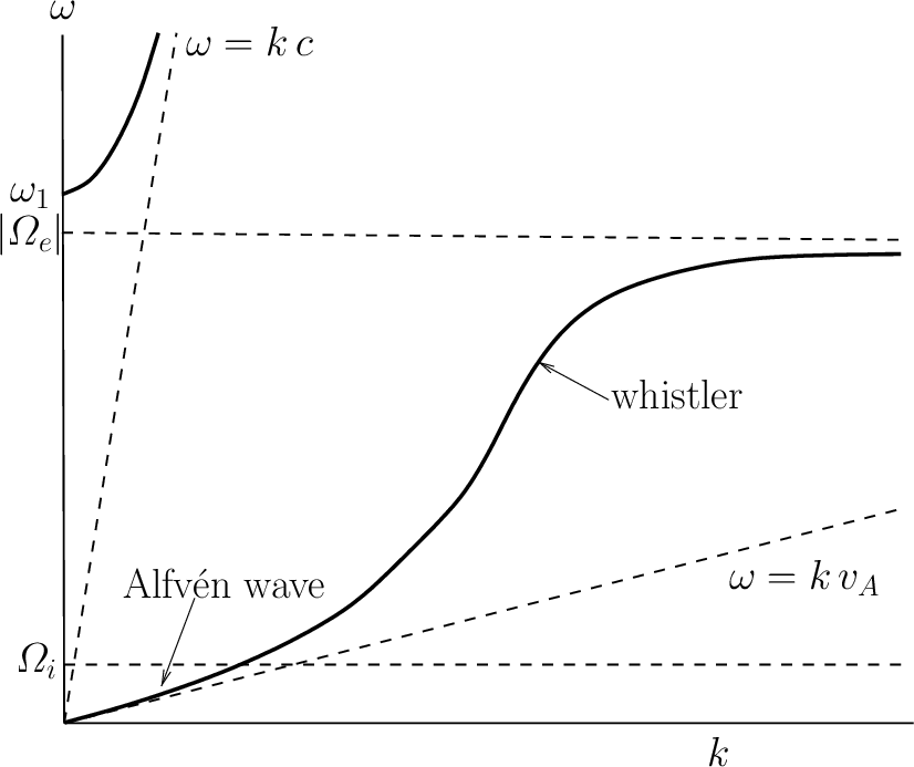
?fig-dispersion-parallel shows the dispersion relations for L/R waves in a rough scale (ACTUALLY THE SCALES ARE SO BAD…). Above the cut-off frequencies (\(\omega_{R=0}\) and \(\omega_{L=0}\)) the solution to the wave dispersion equation is called the free-space mode. Below electron and ion cyclotron frequencies the waves are called the cyclotron modes. At low frequencies (\(\omega\rightarrow 0\)) L- and R-modes merge and the dispersion becomes that of the shear Alfvén wave \(n^2\rightarrow c^2/v_A^2\).

KeyNotes.plot_dispersion_parallel()

The dispersion curve for a R-wave propagating parallel to the equilibrium magnetic field is sketched in Figure 7.2. The continuation of the Alfvén wave above the ion cyclotron frequency is called the electron cyclotron wave, or sometimes the whistler wave. The latter terminology is prevalent in ionospheric and space plasma physics contexts. The phase speed is mostly super-Alfvénic except near the electron gyrofrequency. The wave which propagates above the cutoff frequency, \(\omega_1\), is a standard right-handed circularly polarized electromagnetic wave, somewhat modified by the presence of the plasma. Note that the low-frequency branch of the dispersion curve differs fundamentally from the high-frequency branch, because the former branch corresponds to a wave which can only propagate through the plasma in the presence of an equilibrium magnetic field, whereas the high-frequency branch corresponds to a wave which can propagate in the absence of an equilibrium field.

Figure 7.2: Dispersion relation for a right-handed wave propagating parallel to the magnetic field in a magnetized plasma.

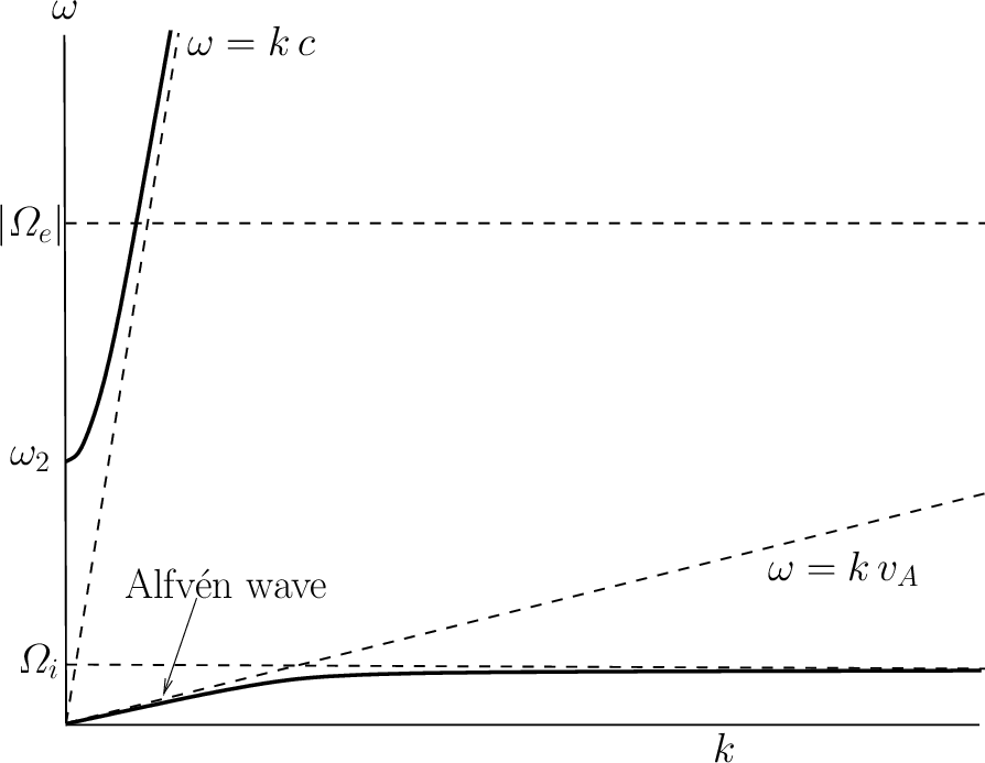
For a L-wave, similar considerations to the above give a dispersion curve of the form sketched in Figure 7.3. In this case, \(n^2\) goes to infinity at the ion cyclotron frequency, \(\Omega_i\), corresponding to the so-called ion cyclotron resonance (at \(L\rightarrow\infty\)). At this resonance, the rotating electric field associated with a left-handed wave resonates with the gyromotion of the ions, allowing wave energy to be converted into perpendicular kinetic energy of the ions. There is a band of frequencies, lying above the ion cyclotron frequency, in which the left-handed wave does not propagate. At very high frequencies a propagating mode exists, which is basically a standard left-handed circularly polarized electromagnetic wave, somewhat modified by the presence of the plasma.

As before, the lower branch in Figure 7.3 describes a wave that can only propagate in the presence of an equilibrium magnetic field, whereas the upper branch describes a wave that can propagate in the absence an equilibrium field. The continuation of the Alfvén wave to just below the ion cyclotron frequency is generally called the ion cyclotron wave. Note that the phase speed is always sub-Alfvénic.

Figure 7.3: Dispersion relation for a left-handed wave propagating parallel to the magnetic field in a magnetized plasma.

7.7.6 Faraday Rotation

A linearly polarized plane wave can be expressed as a sum of left- and right-hand circularly polarized waves (R- and L-modes having equal amplitudes, \(E_0\)). If we assume that at \(z=0\), the wave is linearly polarized along the \(x\)-axis, and that the wave vector \(\mathbf{k}\) and the background magnetic field \(\mathbf{B}_0\) are along the \(z\)-axis, we can write \[ \mathbf{E} = E_0 [(e^{ik_Rz}+e^{ik_Lz})\hat{x} + (e^{ik_Rz}-e^{ik_Lz})\hat{y}] e^{-i\omega t} \]

The ratio of the \(E_x\) and \(E_y\) components is \[ \frac{E_x}{E_y} = \cot\Big( \frac{k_L-k_R}{2}z\Big) \]

Hence, due to different phase speeds of R- and L-modes the linrealy polarized wave that is travelling along a magnetic field will experience the rotation of its plane of polarization. This is called Faraday rotation. The magnitude of the rotation depends on the density and magnetic field of the plasma. Considering frequencies above the plasma frequency one can show that the rate of change in the rotation angle \(\phi\) with the distance travelled (assumed here to be in the \(z\)-direction) is \[ \frac{\mathrm{d}\phi}{\mathrm{d}z} = \frac{-e^3}{2m_e^2\epsilon_0 c\omega^2}n_e B_0 \] and the total rotation from the source to the observer is \[ \phi=\frac{-e^3}{2m_e^2\epsilon_0 c\omega^2}\int_0^d n_e\mathbf{B}\cdot \mathrm{d}\mathbf{s} \] where \(\mathrm{d}\mathbf{s}\) is along the wave propagation path. The total rotation thus depends on both the dnesity and magnetic field of the medium.

Faraday rotation is an important diagnostic tool both in laboratories and in astronomy. It can be used to obtain information of the magnetic field of the cosmic plasma. Note that density has to be known using other methods. On the other hand, if the magnetic field is known, Faraday rotation can give information of the density.

7.7.7 Perpendicular Wave Propagation

Let us now consider wave propagation, at arbitrary frequencies, perpendicular to the equilibrium magnetic field, i.e. \(\theta=90^\circ\).

The cutoff frequencies, at which \(n^2\) goes to zero, are the roots of \(R=0\) and \(L=0\) according to \(n^2=LR/S\). In fact, we have already solved these equations in the previous sections (recall that cutoff frequencies do not depend on \(\theta\)). There are two cutoff frequencies, \(\omega_{R=0}\) and \(\omega_{L=0}\), which are specified by Equation 7.22 and Equation 7.23, respectively.

Let us, next, search for the resonant frequencies, at which \(n^2\) goes to infinity. According to the previous discussions, the resonant frequencies are solutions of \[ S = 1 - \frac{\omega_{pe}^2}{\omega^2 - \Omega_e^2} - \frac{\omega_{pi}^2}{\omega^2 - \Omega_i^2} = 0 \tag{7.26}\]

The roots of this equation can be obtained as follows. First, we note that if the first two terms are equated to zero, we obtain \(\omega=\omega_\mathrm{UH}\), where \[ \omega_\mathrm{UH} \equiv \sqrt{\omega_{pe}^2 + \Omega_e^2} \tag{7.27}\]

If this frequency is substituted into the third term, the result is far less than unity. We conclude that \(\omega_\mathrm{UH}\) is a good approximation to one of the roots of Equation 7.26. To obtain the second root, we make use of the fact that the product of the square of the roots is \[ \Omega_e^2\,\Omega_i^2 + \omega_{pe}^2\,\Omega_i^2 + \omega_{pi}^2\Omega_e^2 \simeq \Omega_e^2 \Omega_i^2 + \omega_{pi}^2\,\Omega_e^2 \]

We, thus, obtain \(\omega= \omega_\mathrm{LH}\), where \[ \omega_\mathrm{LH} \equiv \sqrt{\frac{\Omega_e^2\Omega_i^2 + \omega_{pi}^2\Omega_e^2}{\omega_{pe}^2 + \Omega_e^2}} \tag{7.28}\]

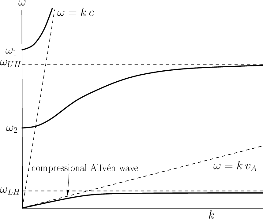
The first resonant frequency, \(\omega_\mathrm{UH}\), is greater than the electron cyclotron or plasma frequencies, and is called the upper hybrid frequency. The second resonant frequency, \(\omega_\mathrm{LH}\), lies between the electron and ion cyclotron frequencies, and is called the lower hybrid frequency. (F. F. Chen 2016) gave some nice explanations of the physical origins of these frequencies by looking at the electrostatic electron/ion waves perpendicular to \(\mathbf{B}\). At low frequencies, the mode in question reverts to the compressional-Alfvén wave discussed previously. Note that the shear-Alfvén wave does not propagate perpendicular to the magnetic field.

Using the above information, and the easily demonstrated fact that \[ \omega_\mathrm{LH} < \omega_{L=0} < \omega_\mathrm{UH} < \omega_{R=0} \]

we can deduce that the dispersion curve for the mode in question takes the form sketched in Figure 7.4. The lowest frequency branch corresponds to the compressional-Alfvén wave. The other two branches constitute the extraordinary, or \(X\)-, wave. The upper branch is basically a linearly polarized (in the \(y\)-direction) electromagnetic wave, somewhat modified by the presence of the plasma. This branch corresponds to a wave which propagates in the absence of an equilibrium magnetic field. The lowest branch corresponds to a wave which does not propagate in the absence of an equilibrium field. Finally, the middle branch corresponds to a wave which converts into an electrostatic plasma wave in the absence of an equilibrium magnetic field.

Figure 7.4: Dispersion relation for a left-handed wave propagating perpendicular to the magnetic field in a magnetized plasma.

Wave propagation at oblique angles is generally more complicated than propagation parallel or perpendicular to the equilibrium magnetic field, but does not involve any new physical effects.

7.8 MHD Waves

7.8.1 Cold MHD

By ignoring pressure, gravity, viscosity and rotation, we have \[ \begin{aligned} \rho \frac{\partial \mathbf{u}}{\partial t} = \mathbf{j}\times\mathbf{B}_0 \\ \mathbf{E} = -\mathbf{u}\times\mathbf{B}_0 \\ \nabla\times\mathbf{E} = -\frac{\partial \mathbf{B}_1}{\partial t} \\ \nabla\cdot\mathbf{B}_1 = 0 \\ \nabla\times\mathbf{B}_1 = \mu_0\mathbf{j} \end{aligned} \tag{7.29}\]

As usual in wave analysis, \(\mathbf{u},\mathbf{j},\mathbf{E}\) are treated as perturbations. The MHD wave equation for the electric field can then be obtained, \[ \begin{aligned} \dot{\mathbf{E}} &= -\dot{\mathbf{u}}\times\mathbf{B}_0 = -\frac{1}{\rho}(\mathbf{j}\times\mathbf{B})\times\mathbf{B}_0 = -\frac{1}{\mu_0\rho}[(\nabla\times\mathbf{B}_1)\times\mathbf{B}_0]\times\mathbf{B}_0 \\ \ddot{\mathbf{E}} &= [(\nabla\times(\nabla\times\mathbf{E}))\times\mathbf{V}_A]\times\mathbf{V}_A \end{aligned} \] where \(\mathbf{V}_A = \mathbf{B}_0 /\sqrt{\mu_0 \rho}\) is the Alfvén velocity, or if we mutate the triad cross terms, \[ \ddot{\mathbf{E}} = \mathbf{V}_A \times [\mathbf{V}_A\times\nabla\times(\nabla\times\mathbf{E})] \tag{7.30}\]

Alternatively, we can also get the MHD wave equation for the magnetic field: \[ \begin{aligned} \left\{ \begin{aligned} \dot{\mathbf{B}_1} = \nabla\times(\mathbf{u}\times\mathbf{B}_0) \\ (\nabla\times\mathbf{B}_1)\times\mathbf{B}_0 = \mu_0\mathbf{j}\times\mathbf{B}_0 = \mu_0\rho\dot{\mathbf{u}} \end{aligned} \right. \\ \Rightarrow \ddot{\mathbf{B}_1} = \nabla\times \Big[ \big( \frac{1}{\mu_0\rho}(\nabla\times\mathbf{B}_1)\times\mathbf{B}_0 \big)\times\mathbf{B}_0 \Big] \end{aligned} \] or \[ \ddot{\mathbf{B}_1} = \nabla\times \Big[ \big( (\nabla\times\mathbf{B}_1)\times\mathbf{V}_A \big)\times\mathbf{V}_A \Big] \tag{7.31}\]

We will see soon that in cold MHD the slow mode ceases to exist, and the fast mode moves at Alfvén speed, such that along the magnetic field line, we only have a single wave mode.

7.8.2 Hot MHD

\[ \begin{aligned} \frac{\partial\rho}{\partial t}+\nabla\cdot(\rho\mathbf{v})=0 \\ \rho\frac{\mathrm{d}\mathbf{v}}{\mathrm{d}t}=-\nabla p+\mathbf{j}\times\mathbf{B} \\ \mathbf{j}=\frac{1}{\mu_0}\nabla\times\mathbf{B} \\ \frac{\mathrm{d}}{\mathrm{d}t}\Big( p\rho^{-\gamma} \Big)=0 \\ \frac{\partial\mathbf{B}}{\partial t}=-\nabla\times\mathbf{E} \\ \mathbf{E}=-\mathbf{v}\times\mathbf{B} \end{aligned} \]

\(\dot{\mathbf{E}}\) is ignored because we only consider low frequency waves. We assume no background flow, \(\mathbf{u}_0=0\), so the current is purely caused by perturbed velocity \(\mathbf{u}_1\). Performing linearization and plane wave decomposition: \[ \begin{aligned} -i\omega\rho_1+i\rho_0\mathbf{k}\cdot\mathbf{v}=0 \\ -i\omega\rho_0\mathbf{v}=-i\mathbf{k}p_1+\mathbf{j}\times\mathbf{B}_0 \\ \mathbf{j}=\frac{1}{\mu_0}i\mathbf{k}\times\mathbf{B}_1 \\ p_1/p_0 -\gamma\rho_1/\rho_0 = 0 \\ -i\omega\mathbf{B}_1=i\mathbf{k}\times(\mathbf{v}\times\mathbf{B}_0) \end{aligned} \]

Let \(\mathbf{B}_0 = B_0\hat{z}\). The linearized equations can be further simplified: \[ \begin{aligned} -i\omega\rho_0\mathbf{v}=-i\mathbf{k}\big( \gamma p_0\frac{\mathbf{k}\cdot\mathbf{v}}{\omega} \big) +\Big[ \frac{1}{\mu_0}i\mathbf{k}\times\big( -\frac{\mathbf{k}\times(\mathbf{v}\times\mathbf{B}_0)}{\omega} \big) \Big]\times\mathbf{B}_0 \\ \omega^2 \mathbf{v}-{v_s}^2 \mathbf{k}(\mathbf{k}\cdot\mathbf{v})-{v_A}^2\big[ \mathbf{k}\times\big( \mathbf{k}\times(\mathbf{v}\times\hat{z})\big) \big]\times\hat{z}=0 \end{aligned} \] where \(v_s=\sqrt{\frac{\gamma p_0}{\rho_0}}\) is the sound speed, and \(v_A=\sqrt{\frac{{B_0}^2}{\mu_0\rho_0}}\) is the Alfvén speed. If we write \(\mathbf{V}_A = \mathbf{B}_0 / \sqrt{\mu_0 \rho_0}\), this can also be written as \[ \omega^2 \mathbf{v} - {v_s}^2 \mathbf{k}(\mathbf{k}\cdot\mathbf{v}) - \mathbf{k}\times \mathbf{k}\times (\mathbf{v}\times\mathbf{V}_A) \times\mathbf{V}_A = 0 \]

Due to the symmetry in the perpendicular x-y plane, for simplicity, we assume the wave vector \(\mathbf{k}\) lies in the x-z plane with an angle w.r.t. the \(z\) axis \(\theta\): \[ \mathbf{k} = k_x\hat{x} + k_z\hat{z} = k_x\hat{x} + k_\parallel\hat{z} = k\sin\theta\hat{x} + k\cos\theta\hat{z} \]

Now it can be written as \[ \begin{pmatrix} -\omega^2/k^2 + v_A^2 + v_s^2\sin^2\theta & 0 & v_s^2\sin\theta\cos\theta \\ 0 & -\omega^2/k^2+v_A^2\cos^2\theta & 0 \\ v_s^2\sin\theta\cos\theta & 0 & -\omega^2/k^2+v_s^2\cos^2\theta \end{pmatrix} \begin{pmatrix} v_x \\ v_y \\ v_z \end{pmatrix} = 0 \tag{7.32}\]

7.8.3 Alfvén Wave

For any nonzero \(v_y\), the \(y\)-component of Equation 7.32 gives \[ \omega^2 = k^2v_A^2\cos^2\theta = k_\parallel^2 v_A^2 \] which is known as the Alfvén wave, in a uniform plasma immersed in a uniform background magnetic field with phase speed \[ v_p = v_A\cos\theta \]

The group velocity and hence energy propagation is always parallel to \(\mathbf{B}\) regardless of the direction of \(\mathbf{k}\), and for this reason this mode is also know as the guided mode. This property, of course, has the direct bearing on the feature of Alfvén wave resonant absorption.

Given the velocity perturbation \(\mathbf{v}_1 = (0, v_y, 0)\), \(-i\omega\rho_1 + \rho_0 \mathbf{k}\cdot\mathbf{v} = 0\), \(\omega\mathbf{B}_1 + \mathbf{k}\times(\mathbf{v}\times\mathbf{B}_0) = 0\), the other perturbations are given as \[ \begin{aligned} \rho_1 &= 0 \\ p_1 &= 0 \\ \mathbf{E} &= -B_0 v_y\hat{x} \\ \mathbf{B}_1 &= \frac{\mathbf{k}}{\omega}\times\mathbf{E} = -\frac{k_zB_0v_y}{\omega}\hat{y} = -\frac{\mathbf{v}}{\omega/k_\parallel}B_0 \\ \mathbf{j} &= \frac{1}{\mu_0}\nabla\times\mathbf{B}_1 = \frac{i\mathbf{k}\times\mathbf{B}_1}{\mu_0} \end{aligned} \tag{7.33}\]

SAW has a wave vector \(\mathbf{k}\) in the XZ-plane. \(\mathbf{E}\) shall oscillate in the X-direction; \(\mathbf{B}\) shall oscillate in the Y-direction. The electric current of the wave \(\mathbf{j}\) lies in the XZ-plane. The timescale of the variations of the wave fields is much longer than the ion gyroperiod \(\Omega_i^{-1}\). In both the perpendicular and parallel directions, the spatial scale of the waves \(1/k\) are much larger than ion motion scale \(r_{iL}\). The wave carries a Poynting flux \(\mathbf{S} = \mathbf{E}\times\mathbf{B}_1\) strictly parallel to \(\mathbf{B}_0\). The ratio of the wave electric field to the wave magnetic field \(|\mathbf{E}|/|\mathbf{B}_1|\) is exactly one Alfvén speed \(V_A\).

\(\mathbf{E}\) (or \(\mathbf{B}_1\)) in Equation 7.33 shows that the Alfvén wave in a uniform plasma is a linearly polarized wave if \(\mathbf{v}_1 = (0, v_y, 0)\). If instead we set \(\mathbf{k}=(0,0,k)\) (\(\theta=0^\circ\)) and \(\mathbf{v}_1 = (v_x, v_y, 0)\), then \(\mathbf{k}\cdot\mathbf{v}=0\Rightarrow \rho_1=0\) but \(\mathbf{E}=-\mathbf{v}\times\mathbf{B}_0 = kv_y\hat{x} - kv_x\hat{y}\) can be a circularly polarized wave or else. Correlated \(\mathbf{B}_1\) and \(\mathbf{v}\) corresponds to waves propagating anti-parallel to the \(\mathbf{B}_0\) (\(\mathbf{k}\cdot\mathbf{B}_0<0\)), and anti-correlated \(\mathbf{B}_1\) and \(\mathbf{v}\) corresponds to waves propagating parallel to the \(\mathbf{B}_0\) (\(\mathbf{k}\cdot\mathbf{B}_0>0\)). (This is the same as expressed by the Alfvénicity condition Equation 15.4.) The resultant magnetic field then exhibits shear, thus the Alfvén wave is called the shear Alfvén wave (SAW). An animation of SAW is shown in Figure 7.5.

Figure 7.5: Alfvén wave.

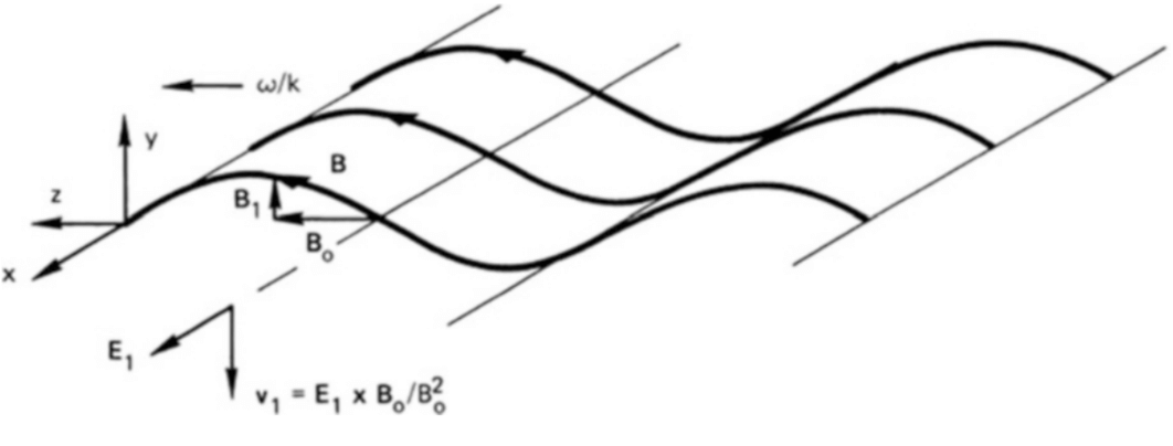
To understand what happens physically in an Alfvén wave, recall that this is an electromagnetic wave with a fluctuating magnetic field \(\mathbf{B}_1\) given by \[ \nabla\times\mathbf{E}_1 = -\dot{\mathbf{B}}_1\quad E_x=(\omega/k)B_y \tag{7.34}\]

The small component \(B_y\), when added to \(\mathbf{B}_0\), gives the magnetic field lines a sinuisoidal ripple, shown exaggerated in Figure 7.6. At the point shown, \(B_y\) is in the positive \(y\) direction, so, according to Equation 7.34, \(E_x\) is in the positive \(x\) direction if \(\omega/k\) is in the \(z\) direction. The electric field \(E_x\) gives the plasma an \(\mathbf{E}_1\times\mathbf{B}_0\) drift in the negative \(y\) direction. Since we have taken the limit \(\omega^2\ll\Omega_{c}\), both ions and electrons will have the same drift \(v_y\), obtained from Section 7.7 the component \(v_y\) under \(T_i=0\): \[ \begin{aligned} v_{ix} &= \frac{iq}{m \omega}\left( 1-\frac{\Omega_c^2}{\omega^2} \right)^{-1} E_1 \\ v_{iy} &= \frac{q}{m\omega}\frac{\Omega_c}{\omega} \left( 1-\frac{\Omega_c^2}{\omega^2} \right)^{-1} E_1 \end{aligned} \tag{7.35}\]

Thus, the fluid moves up and down in the y direction. The magnitude of this velocity is \(|E_x/B_0|\). Since the ripple in the field is moving by at the phase velocity \(\omega/k\), the magnetic field is also moving downward at the point indicated in Figure 7.6. The downward velocity of the magnetic field lines is \((\omega/k)|B_y/B_0|\), which, according Equation 7.34, is just equal to the fluid velocity \(|E_x/B_0|\). Thus, the fluid and the field lines oscillate together as if the particles were stuck to the lines. The magnetic field lines act as if they were mass-loaded strings under tension, and an Alfvén wave can be regarded as the propagating disturbance occurring when the strings are plucked. This concept of plasma frozen to the field lines and moving with them is a useful one for understanding many low-frequency plasma phenomena. It can be shown that this notion is an accurate one as long as there is no electric field along \(\mathbf{B}\).

Figure 7.6: Relation among the oscillating quantities in an Alfvén wave and the (exaggerated) distortion of the lines of force.

It remains for us to see what sustains the electric field \(E_x\) which we presupposed was there. As \(\mathbf{E}_1\) fluctuates, the ions’ inertia causes them to lag behind the electrons, and there is a polarization drift \(\mathbf{v}_p\) in the direction of \(\mathbf{E}_1\). This drift \(v_{ix}\) is given by Equation 7.35 and causes a current \(\mathbf{j}_1\) to flow in the \(x\) direction. The resulting \(\mathbf{j}_1\times\mathbf{B}_0\) force on the fluid is in the \(y\) direction and is \(90^\circ\) out of phase with the velocity \(\mathbf{v}_1\). This force perpetuates the oscillation in the same way as in any oscillator where the force is out of phase with the velocity. It is, of course, always the ion inertia that causes an overshoot and a sustained oscillation, but in a plasma the momentum is transferred in a complicated way via the electromagnetic forces.

In a more realistic geometry for experiments, \(\mathbf{E}_1\) would be in the radial direction and \(\mathbf{v}_1\) in the azimuthal direction. The motion of the plasma is then incompressible. This is the reason the \(\nabla p\) term in the equation of motion could be neglected.

In a non-uniform plasma, SAW attains the interesting property of a continuous spectrum. To illustrate this feature, let us consider the simplified slab model of a cold plasma with a non-uniform density, \(\rho=\rho(x)\), and a uniform \(\mathbf{B}_0 = B_0\hat{z}\). Assuming at \(t=0\) a localized initial perturbation \(\mathbf{B}_{1y}(x,t=0) = \exp(-x^2/\Delta x^2)\), \(|k_y\Delta_x|\ll1\), and \(\partial\mathbf{B}_{1y}/\partial t=0\), the perturbation then evolves according to the following wave equation (Equation 7.31, \(B_{1z}=0\) so no coupling between the fast mode and Alfvén mode): \[ [\partial_t^2 + \omega_A^2(x)]B_{1y}(x,t) = 0 \]

Here \(\omega_A^2(x) = k_z^2v_A^2(x)\) and the solution is \[ B_{1y}(x,t) = \hat{B}_{1y}(x,0)\cos[\omega_A(x)t] \tag{7.36}\]

Equation 7.36 shows that every point in \(x\) oscillates at a different frequency, \(\omega_A(x)\). With a continuously varying \(\omega_A(x)\); the wave frequency, thus, constitutes a continuous spectrum. While the above result is based on a model with a 1D non-uniformity in x, this general feature of SAW continuous spectrum also holds in magnetized plasmas with 2D or 3D non-uniformities. A good example is geomagnetic pulsations in the Earth’s magnetosphere observed by Engebretson shown in Figure 1 of (L. Chen, Zonca, and Lin 2021).

Equation 7.36 also indicates an unique and important property of SAW continuous spectrum: the spatial structure evolves with time. Specifically, the wave number in the non-uniformity direction is, time asymptotically, given by: \[ |k_x| = \bigg\lvert\frac{\partial \ln B_{1y}}{\partial x}\bigg\rvert \simeq \bigg\lvert\frac{\mathrm{d} \omega_A(x)}{\mathrm{d} x}\bigg\rvert t \tag{7.37}\]

That \(|k_x|\) increases with \(t\) is significant, since it implies that any initially long-scale perturbations will evolve into short scales. This point is illustrated in Figure ??? (CAN I PERFORM THE SIMULATION?); showing the evolution of a smooth \(B_{1y}\) at \(t=0\) to a spatially fast varying \(B_{1y}\) at a later \(t\).

Another consequence of \(|k_x|\) increasing with \(t\) is the temporal decay of \(B_{1x}\). From \(\nabla\cdot\mathbf{B}_1 \simeq \nabla_\perp\cdot\mathbf{B}_{1\perp}=0\), we can readily derive that, for \(|\omega_A^\prime t|\gg |k_y|\): \[ B_{1x}(x, t)\simeq \frac{k_y}{\omega_A^\prime(x)t}\hat{B}_{1y}(x,0)e^{-i\omega_A(x)t}\Big[ 1+\mathcal{O}\Big( \frac{k_y}{|\omega_A^\prime t|+ ...} \Big) \Big] \]

That is, \(B_{1x}\) decays temporally due to the phase mixing of increasingly more rapidly varying neighboring perturbations.

Noting that, as \(t\rightarrow\infty\), \(|k_x|\rightarrow\infty\), it thus suggests that the perturbation will develop singular structures toward the steady state. As we will see in the field line resonance Chapter 13, the singularity is reached at the Alfvén resonant point \(x_r\), where \(\omega^2=\omega_A^2(x_r)\) along with a finite resonant wave-energy absorption rate. Note that at the isolated extrema of the SAW continuum, \(|\omega_A^\prime|=0\), phase mixing vanishes; consequently, perturbation remains regular and experiences no damping via resonant absorption. This feature has important implications to Alfvén instabilities in laboratory plasmas.

Space plasmas support a variety of waves, but for heating the plasma and accelerating the electrons and ions, Alfvén waves are a predominant source. Near the Sun, Alfvén waves are excited and propagate outward. They exchange their energy with particles to accelerate them in the form of solar wind and heat the electrons. When perpendicular wavelength of the wave becomes comparable to the ion gyro-radius (\(k_\perp r_{Li}\sim 1\)) or inertial length (\(k_\perp d_i \sim 1\)) in the case of kinetic Alfvén waves (KAWs, Section 7.9.4) or inertial Alfvén waves (IAWs, Equation 7.71), respectively, then the wave in both the limits has a nonzero parallel electric field component which is responsible for the acceleration of the particles via the Landau mechanism. This is also consistent with the generalized Ohm’s law Equation 5.27: only when we go beyond Hall MHD can \(\mathbf{E}_\parallel\) be nonzero. (WHAT ABOUT \(\eta\mathbf{j}\)?) KAW relates to \(\frac{\nabla P_e}{ne}\) term, while IAW relates to \(\frac{\partial \mathbf{j}}{\partial t}\) term. The key interest is in \(E_\parallel\). KAWs and IAWs have significance not only in space plasmas but also in laboratory plasma such as in fusion reactors.

Alfvén wave has very high saturation level, meaning that it takes a long time for the wave to reach the nonlinear phase. (???)

SAW in a Slab

We now look deeper into the properties of Alfvén waves in a nonuniform magnetized plasma slab that carries a current flowing along an externally imposed magnetic field \(B_{0z}\hat{z}\), where \(B_{0z}\) is assumed to be a constant. First, we formulate the governing equation for the slab geometry, under the ideal MHD condition. Then we show that Alfvén waves are always neutrally stable, with important indication at the end.

The presence of an equilibrium current density \(\mathbf{J}_0 = \widehat{z}J_0(x)\) produces a local magnetic field of the form \[ \mathbf{B}_0 = \hat{z}B_{0z} + \hat{y}B_{0y}(x) \]

The Ampère’s law gives \[ \nabla\times\mathbf{B}_0 = \mu_0 \mathbf{J}_0 \Rightarrow \frac{\partial B_{0y}}{\partial x}-\frac{\partial B_{0x}}{\partial y} = \frac{\partial B_{0y}}{\partial x} = \mu_0 J_0(x) \tag{7.38}\]

From the force balance equation, \[ \mathbf{J}_0\times\mathbf{B}_0 = \nabla P_0 \tag{7.39}\]

Substituting Equation 7.38 into Equation 7.39, we get \[ \frac{{B_{0y}(x)}^2}{2\mu_0} + P_0(x) = \text{const.} \]

Designate all perturbation quantities with a subscript 1, and assume \(e^{-i\omega t+ik_y y+ i k_z z}\) dependence for all perturbations (nonuniform in the \(x\)-direction, thus no sinuisoidal wave assumption). From linearized Faraday’s law and Ohm’s law in ideal MHD,

\[ \begin{aligned} -\nabla\times\mathbf{E}_1 = \nabla\times(\mathbf{v}_1\times\mathbf{B}_0) = \frac{\partial\mathbf{B}_1}{\partial t} \\ -i\omega\mathbf{B}_1 = \mathbf{v}_1\cancel{(\nabla\cdot\mathbf{B}_0)}-\mathbf{B}_0\cancel{(\nabla\cdot\mathbf{v}_1)}+(\mathbf{B}_0\cdot\nabla) \mathbf{v}_1 - (\mathbf{v}_1\cdot\nabla)\mathbf{B}_0 \end{aligned} \] where we have assumed the plasma is incompressible. Replace \(\nabla\) with \(i\mathbf{k}\), \(\mathbf{v}_1=i\omega \pmb{\xi}_1\) and take the \(x\)-component, we get \[ B_{1x} = i(\mathbf{k}\cdot\mathbf{B}_0)\xi_{1x} \tag{7.40}\] where \(\mathbf{k}=\hat{y}k_y+\hat{z}k_z\).

The MHD force law can be linearized to \[ \rho_0 \frac{\partial \mathbf{v}_1}{\partial t} = -\nabla\Big( p_1 + \frac{\mathbf{B}_0\cdot\mathbf{B}_1}{\mu_0}\Big) + \frac{1}{\mu_0}\big[ (\mathbf{B}_0\cdot\nabla)\mathbf{B}_1 + (\mathbf{B}_1\cdot\nabla)\mathbf{B}_0\big] \tag{7.41}\]

Since the plasma is incompressible, \(\nabla\cdot\pmb{v}_1=0,\ \dot{\pmb{\xi}}=\mathbf{v}_1\Rightarrow \nabla\cdot\pmb{\xi}=0\). In addition, \(\nabla\cdot\mathbf{B}_1=0\). We then have \[ \begin{aligned} \mathbf{k}\cdot\pmb{\xi}_{1yz}&=i\frac{\partial \xi_{1x}}{\partial x} \\ \mathbf{k}\cdot\pmb{B}_{1yz}&=i\frac{\partial B_{1x}}{\partial x} \end{aligned} \] where \(\pmb{\xi}_{1yz} = (0,\xi_{1y},\xi_{1z})\), \(\mathbf{B}_{1yz}=(0,B_{1y},B_{1z})\). The \(x\)-component of Equation 7.41 gives \[ -\rho_0\omega^2 \xi_{1x} = -\frac{\partial}{\partial x}\Big( p_1 + \frac{\mathbf{B}_0\cdot\mathbf{B}_1}{\mu_0}\Big) +\frac{1}{\mu_0} \big[ (\mathbf{B}_0\cdot\nabla)B_{1x} \big] \tag{7.42}\]

The dot product of Equation 7.41 with \(\mathbf{k}\) gives \[ \begin{aligned} -\rho_0 \omega^2 \mathbf{k}\cdot\pmb{\xi}_{1yz} &= ik^2 \Big( p_1 + \frac{\mathbf{B}_0\cdot\mathbf{B}_1}{\mu_0}\Big) + \frac{1}{\mu_0}\big[ i(\mathbf{k}\cdot\mathbf{B}_0)(\mathbf{k}\cdot\mathbf{B}_{1yz}) + B_{1x}\frac{\partial }{\partial x}(\mathbf{k}\cdot\mathbf{B}_0)\big]\\ -\rho_0 \omega^2 i\frac{\partial \xi_{1x}}{\partial x} &= ik^2 \Big( p_1 + \frac{\mathbf{B}_0\cdot\mathbf{B}_1}{\mu_0}\Big) + \frac{1}{\mu_0}\big[ i(\mathbf{k}\cdot\mathbf{B}_0)(i\frac{\partial B_{1x}}{\partial x}) + B_{1x}\frac{\partial }{\partial x}(\mathbf{k}\cdot\mathbf{B}_0)\big] \end{aligned} \tag{7.43}\]

Finally, canceling \(p_1 + \frac{\mathbf{B}_0\cdot\mathbf{B}_1}{\mu_0}\) from Equation 7.42 and Equation 7.43 and substituting \(B_{1x}\) from Equation 7.40, we obtain the governing equation \[ \frac{\partial}{\partial x}\Big\{ \rho_0 \big[ \omega^2 - (\mathbf{k}\cdot\mathbf{v}_A)^2\big]\frac{\partial \xi_{1x}}{\partial x}\Big\} -k^2\rho_0 \big[ \omega^2 - (\mathbf{k}\cdot\mathbf{v}_A)^2\big]\xi_{1x}=0 \tag{7.44}\] where \(k^2={k_y}^2+ {k_z}^2\), \(\mathbf{v}_A = v_A \mathbf{B}_0/B_0\), and \(v_A=B_0/\sqrt{\mu_0 \rho_0}\) is the local Alfvén speed. This is the governing equation of shear Alfvén waves in a slab geometry derived by Hasegawa and Liu Chen in the 1970s, which is readily compared with Eq.(10.33) in (Bellan 2008).

It is easy to show that this governing equation always yields neutrally stable solutions of SAWs, i.e. \(\omega_i=\Im(\omega)=0\). Multiply it by \(\xi_{1x}^\ast\), and integrate the resultant equation to get \[ \int_{-\infty}^{\infty}\mathrm{d}x \rho_0 \big[ \omega^2-(\mathbf{k}\cdot\mathbf{v}_A)^2\big] \Big[ \bigg\lvert \frac{\mathrm{d}\xi_{1x}}{\mathrm{d}x}\bigg\rvert^2 + k^2\lvert\xi_{1x}\rvert^2 \Big] = 0 \] where we have assumed that \(\xi_{1x}\) vanishes on the boundary. This gives \[ \omega^2 = \frac{\int_{-\infty}^{\infty}\mathrm{d}x \rho_0 (\mathbf{k}\cdot\mathbf{v}_A)^2\Big[ \bigg\lvert \frac{\mathrm{d}\xi_{1x}}{\mathrm{d}x}\bigg\rvert^2 + k^2\lvert \xi_{1x}\rvert^2 \Big]}{\int_{-\infty}^{\infty}\rho_0[ \lvert \frac{\mathrm{d}\xi_{1x}}{\mathrm{d}x}\rvert^2 + k^2\lvert \xi_{1x}\rvert^2]\mathrm{d}x} \ge 0 \]

SAWs are the dominant low frequency waves in a current carrying plasma. The neutrally stable modes studies above can be destabilized by unfavorable curvature, and such modes are called ballooning modes (Section 10.7.4). They may also be destabilized by a finite electrical resistivity, and these are tearing modes (Section 10.7.5). Their interaction with fusion-generated alpha particles are a major issue in all magnetic fusion schemes. Finally, since the governing equation exhibits a singularity when \(\omega=\mathbf{k}\cdot\mathbf{v}_A\), this singularity represents resonance absorption, which forms the basis of Alfvén wave heating (i.e. field line resonance, Chapter 13). This singularity also give rise to the so called “Alfvén continuum spectrum” mentioned above.

Note that the governing equation is valid even if \(B_{0z}\) is an arbitrary function of \(x\). If in addition, an external gravity \(\mathbf{g}=\hat{x}g\) in the x-direction is present, the governing equation is modified simply by inserting the term \(-(g/\rho_0)\mathrm{d}\rho_0/\mathrm{d}x\) in the second square bracket, and the equation is identical to Eq.(10.33) of Bellan. This is the most general equation which describes the magneto-Rayleigh-Taylor instability (MRT) in Cartesian geometry using the incompressible, ideal MHD model.

7.8.4 Fast and Slow Wave

The \(x\)-\(z\) components of Equation 7.32 give \[ \begin{aligned} (\omega^2-k^2{v_A}^2-{k_x}^2{v_s}^2)v_x -k_x k_z{v_x}^2v_z = 0 \\ (\omega^2-{k_z}^2{v_s}^2)v_z -k_x k_z{v_s}^2v_x=0 \end{aligned} \]

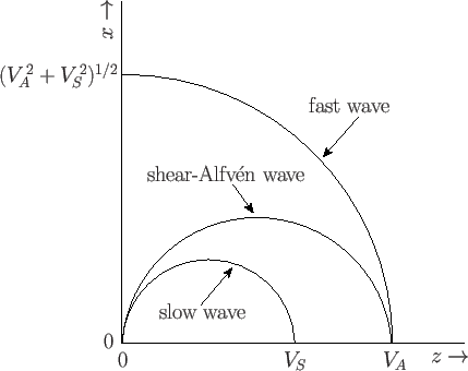
The dispersion relation is given by the determinant being 0, \[ \begin{aligned} \omega^4-k^2({v_A}^2+{v_s}^2)\omega^2+{k_z}^2{v_s}^2k^2{v_A}^2=0 \\ \frac{\omega^2}{k^2}=\frac{1}{2}({v_A}^2+{v_s}^2)\pm\frac{1}{2}\sqrt{({v_A}^2+{v_s}^2)^2-4{v_s}^2{v_A}^2\cos^2\theta} \end{aligned} \tag{7.45}\]

“+” corresponds to the fast mode, or magnetosonic mode, and “-” corresponds to the slow mode. The Friedrich graph Figure 7.7 is very useful in interpreting Equation 7.45. Here we only show the case for \(v_A>v_s\); if \(v_A<v_S\), then along the background magnetic field direction \(\hat{z}\) the fast wave will have a phase speed \(v_\mathrm{ph} = v_s\), and the slow wave will a phase speed \(v_\mathrm{ph} = v_A\) that overlaps with the Alfvén wave. Thus in the high-\(\beta\) case slow wave may have a faster phase speed than the Alfvén wave at a proper angle!

Another thing to be careful about is that when you observe a wave propagating at the Alfvén speed along the field line, you need more information to determine the characteristics of the wave:

• Check the \(\beta\)-regime as well as the compressionality to determine if it has fast/slow wave component.
• Check the polarization to see if it is an cyclotron wave.
• Check the parallel electric field to see if has kinetic features.

Figure 7.7: Friedrich diagram showing the variation of the phase velocities of the three MHD waves with direction of propagation in the x-z plane when \(v_A>v_s\), i.e. low-\(\beta\) case.

Given the velocity perturbation \(\mathbf{v}_1 = (v_x, 0, v_z)\), the other perturbations are given as \[ \begin{aligned} \rho_1 &= \frac{\rho_0}{\omega}\mathbf{k}\cdot\mathbf{v} \\ p_1 &= \gamma p_0\frac{\rho_1}{\rho_0} = \frac{\gamma p_0}{\omega}\mathbf{k}\cdot\mathbf{v} \\ \mathbf{E} &= B_0 v_x\hat{y} \\ \mathbf{B}_1 &= \frac{\mathbf{k}}{\omega}\times\mathbf{E} = \frac{(\mathbf{k}\cdot\mathbf{v})\mathbf{B}_0 - (\mathbf{k}\cdot\mathbf{B}_0)\mathbf{v}}{\omega} = -\frac{B_0 v_x k_z}{\omega}\hat{x} + \frac{B_0v_xk_x}{\omega}\hat{z} \\ \mathbf{j} &= \frac{1}{\mu_0}\nabla\times\mathbf{B}_1 = \frac{i\mathbf{k}\times\mathbf{B}_1}{\mu_0} \end{aligned} \tag{7.46}\]

\(\mathbf{E}\) shows that the fast/slow modes in a uniform plasma are also linearly polarized. When we have \(\theta=90^\circ\) (Figure 7.8), the magnetic perturbation can be simplified to \[ \mathbf{B}_1 = \frac{v}{\omega/k_\perp}\mathbf{B}_0 \] which means that the perturbed magnetic field is always aligned with the background magnetic field.

The distinction between the fast and slow waves can be further understood by comparing the signs of the wave induced fluctuations in the plasma and magnetic pressures: \(p\) and \(\mathbf{B}_0\cdot\mathbf{B}/\mu_0\), respectively. It follows from Equation 7.46 that \[ \frac{\mathbf{B}_0\cdot\mathbf{B}}{\mu_0} = \frac{\mathbf{k}\cdot\mathbf{v}B_0^2 - (\mathbf{k}\cdot\mathbf{B}_0)(\mathbf{B}_0\cdot\mathbf{v})}{\mu_0\,\omega} \]

The \(z\)-component of the perturbed momentum equation yields \[ \omega\rho_0 v_z = k \cos\theta p \]

Combining the above, we have \[ \frac{\mathbf{B}_0\cdot\mathbf{B}}{\mu_0} = \frac{v_A^2}{v_s^2}\left( 1 - \frac{k^2 v_s^2\cos^2\theta}{\omega^2} \right) p \tag{7.47}\]

Hence, \(p\) and \(\mathbf{B}_0\cdot\mathbf{B}/\mu_0\) have the same sign if \(V_\mathrm{ph}=\omega/k>v_s \,\cos\theta\), and the opposite sign if \(V_\mathrm{ph}<v_s\,\cos\theta\). It is straightforward to show that \(v_+> v_s\,\cos\theta\), and \(v_-<v_s\,\cos\theta\). Thus, we conclude that in the fast magnetosonic wave the pressure and magnetic energy fluctuations reinforce one another, whereas the fluctuations oppose one another in the slow magnetosonic wave.

The temperature perturbation, based on the equation of state, can be derived as follows: \[ \begin{aligned} T_1 &= T - T_0 = \frac{p_0 + p_1}{(n_0 + n_1)k_B} - \frac{p_0}{n_0 k_B} \\ &= p_0\left( 1+\gamma\frac{n_1}{n_0} \right) \frac{1}{(n_0 + n_1)k_B} - \frac{p_0}{n_0 k_B} \\ &= p_0\frac{1}{k_B}\left[ \left(1+\gamma\frac{n_1}{n_0}\right)\frac{1}{n_0 + n_1} - \frac{1}{n_0} \right] \\ &= p_0\frac{1}{k_B}\left[ \frac{(\gamma-1)n_1}{n_0(n_0+n_1)} \right] \\ &= T_0\left(\gamma-1 \right)\frac{\mathbf{k}\cdot\mathbf{v}}{\omega + \mathbf{k}\cdot\mathbf{v}} \end{aligned} \tag{7.48}\]

Equation 7.48 shows that temperature does not follow the same sinusoidal shape as the perturbed velocity.

Special attention is required for the extreme cases. When \(\theta=90^\circ\), the fast wave phase speed \(v_\mathrm{ph}=\sqrt{v_A^2 + v_s^2}\) while the slow wave phase speed \(v_\mathrm{ph}=0\). Slow waves cannot propagate perpendicular to the magnetic field. However, this is still a valid solution with all the slow mode perturbation properties, and you will see in Section 10.11.2 and Section 11.2 that this is named mirror mode. When \(\theta=0^\circ\), the fast wave phase speed \(v_\mathrm{ph}=\max(v_A, v_s)\) while the slow wave phase speed \(v_\mathrm{ph}=\min(v_A, v_s)\).

It is important to understand the nature of fast and slow waves under the cold plasma limit, i.e. in the low-\(\beta\) regime where \(v_A\gg v_s\) (cold, strong B). If \(v_s\rightarrow 0\), the slow mode ceases to exit (\(V_\mathrm{ph}\rightarrow 0\)) and the phase speed of the fast mode becomes \(v_p \approx v_A\). This is often called the compressional Alfvén wave, which is actually a fast wave in the low-\(\beta\) limit. If \(\beta\) is low but we still have a finite sound speed, the dispersion relation for the slow wave reduces to \[ \omega \simeq k\,v_s\,\cos\theta \]

Thus, in low-\(\beta\) plasmas the slow wave is a sound wave modified by the presence of the magnetic field.

Figure 7.8: Fast wave.

Sometimes the fast wave dispersion relation is written in alternative ways. Let \(a=\omega/(k_\parallel v_A)=\omega/(k\cos\theta\,v_A)\). From Equation 7.45, we have \[ \cos^2\theta = \frac{a^2\left( v_s^2/v_A^2 + 1 \right)-v_s^2/v_A^2}{a^4} \tag{7.49}\]

This expression is useful when considering the wave resonance and mode conversions. For example, Alfvén resonance occurs when \[ \omega^2 = k_\parallel^2 v_A^2 \tag{7.50}\] i.e. \(a=1\) under the low frequency approximation. In higher frequency cases, the Alfvén resonance condition is modified as \[ a = \frac{1}{\left( 1-\omega^2/\Omega_i^2 \right)^2} \tag{7.51}\] because of the finite ion Larmor radius effects. (The Alfvén resonance singularity can be removed by including non‐MHD effects such as electron inertia or ion Larmor radius corrections.)

7.8.5 Limitations of the MHD model

The MHD model ignores parallel electron dynamics and so has a shear mode dispersion \(\omega^2=k_z^2 v_A^2\) that has no dependence on \(k_\perp\). Some researchers interpret this as a license to allow arbitrarily large \(k_\perp\) in which case a shear mode could be localized to a single field line. However, the two-fluid model of the shear mode does have a dependence on \(k_\perp\) which becomes important when either \(k_\perp c/\omega_{pe}\) or \(k_\perp r_{Ls}\) become of order unity (whether to use \(c\omega_{pe}\) or \(r_{Ls}\) depends on whether \(\beta m_i/m_e\) is small or large compared to unity). Since \(c\omega_{pe}\) and \(r_{Ls}\) are typically small lengths, the MHD point of view is acceptable provided the characteristic length of perpendicular localization is much larger than \(c\omega_{pe}\) or \(r_{Ls}\).

MHD also predicts a sound wave which is identical to the ordinary hydrodynamic sound wave of an unmagnetized gas. The perpendicular behavior of this sound wave is consistent with the two-fluid model because both two-fluid and MHD perpendicular motions involve compressional behavior associated with having finite \(B_{z1}\). However, the parallel behavior of the MHD sound wave is problematical because \(E_{z1}\) is assumed to be identically zero in MHD. According to the two-fluid model, any parallel acceleration requires a parallel electric field. The two-fluid \(B_{z1}\) mode is decoupled from the two-fluid \(E_{z1}\) mode so that the two-fluid \(B_{z1}\) mode is both compressional and has no parallel motion associated with it.

The MHD analysis makes no restriction on the electron to ion temperature ratio and predicts that a sound wave would exist for \(T_e = T_i\). In contrast, the two-fluid model shows that sound waves can only exist when \(T_e \gg T_i\) because only in this regime is it possible to have \(k_B T_i /m_i \ll \omega^2 / k_z^2 \ll k_B T_e /m_e\) and so have inertial behavior for ions and kinetic behavior for electrons.

Various paradoxes develop in the MHD treatment of the shear mode but not in the two-fluid description. These paradoxes illustrate the limitations of the MHD description of a plasma and shows that MHD results must be treated with caution for the shear (slow) mode. MHD provides an adequate description of the fast (compressional) mode.

7.9 Two-fluid model of Alfvén modes

We now examine the MHD modes from a two-fluid point of view. The two-fluid point of view shows that the shear mode occurs as one of two distinct modes, only one of which can exist for given plasma parameters. Which of these shear modes occurs depends upon the ratio of hydrodynamic pressure to magnetic pressure. This ratio is defined for each species s as \[ \beta_s = \frac{n k_B T_s}{B^2/\mu_0} \] The subscript s is not used if electrons and ions have the same temperature. \(\beta_i\) measures the ratio of ion thermal velocity to the Alfvén velocity since \[ \frac{v_{Ti}^2}{v_A^2} = \frac{k_B T_i/m_i}{B^2/nm_i\mu_0} = \beta_i \]

Thus, \(v_{Ti}\ll v_A\) corresponds to \(\beta_i\ll 1\). Magnetic forces dominate hydrodynamic forces in a low \(\beta\) plasma, whereas in a high \(\beta\) plasma the opposite is true.

The ratio of electron thermal velocity to Alfvén velocity is also of interest and is \[ \frac{v_{Te}^2}{v_A^2} = \frac{k_B T_e/m_e}{B^2/nm_i\mu_0} = \frac{m_i}{m_e}\beta_e \]

Thus, \(v_{Te}^2\gg v_A^2\) when \(\beta_e\gg m_e/m_i\) and \(v_{Te}^2\ll v_A^2\) when \(\beta_e\ll m_e/m_i\). Shear Alfvén wave physics is different in the \(\beta_e\gg m_e/m_i\) and \(\beta_e\ll m_e/m_i\) regimes which therefore must be investigated separately. MHD ignores this \(\beta_e\) dependence, an oversimplification which leads to the paradoxes.

Both Faraday’s law and the pre-Maxwell Ampère’s law (no displacement current) are fundamental to Alfvén wave dynamics. The system of linearized equations thus is \[ \begin{aligned} \nabla\times\mathbf{E}_1 = -\frac{\partial\mathbf{B}_1}{\partial t} \\ \nabla\times\mathbf{B}_1 = \mu_0 \mathbf{j}_1 \end{aligned} \tag{7.52}\]

If the dependence of \(\mathbf{j}_1\) on \(\mathbf{E}_1\) can be determined, then the combination of Ampère’s law and Faraday’s law provides a complete self-consistent description of the coupled fields \(\mathbf{E}_1, \mathbf{B}_1\) and hence describes the normal modes. From a mathematical point of view, specifying \(\mathbf{j}_1(\mathbf{E}_1)\) means that there are as many equations as dependent variables in the pair of Equation 7.52. The relationship between \(\mathbf{j}_1\) and \(\mathbf{E}_1\) is determined by the Lorentz equation or some generalization thereof (e.g., drift equations, Vlasov equation, fluid equation of motion). The MHD derivation used the polarization drift to give a relationship between \(j_{1\perp}\) and \(E_{1\perp}\) but leaves ambiguous the relationship between \(j_{1\parallel}\) and \(E_{1\parallel}\).

The two-fluid equations provide a definite description of the relationship between \(j_{1\parallel}\) and \(E_{1\parallel}\). At frequencies well below the cyclotron frequency, decoupling of modes also occurs in the two-fluid description, and this decoupling is more clearly defined and more symmetric than in MHD. The decoupling in a uniform plasma results because the dependence of \(\mathbf{j}_1\) on \(\mathbf{E}_1\) has the property that \(j_{1z}\sim E_{1z}\) and \(\mathbf{j}_{1\perp}\sim\mathbf{E}_{1\perp}\). Thus, for \(\omega\ll\omega_{ci}\) there is a simple linear relation between parallel electric field and parallel current and another distinct simple linear relation between perpendicular electric field and perpendicular current; these two linear relations mean that the tensor relating \(\mathbf{j}_1\) to \(\mathbf{E}_1\) is diagonal (at higher frequencies this is not the case). The decoupling can be seen by supposing that all first order quantities have the dependence \(\exp(i\mathbf{k}_\perp\cdot\mathbf{x}+ik_z z)\) where \(\mathbf{k}_\perp = k_x\hat{x}+k_y\hat{y}\). Mode decoupling can be seen by examining Table 7.1 which lists the electric and magnetic field components:

Table 7.1: Parallel and perpendicular mode decoupling

\(\mathbf{E}\) components	\(\mathbf{B}\) components
* \(\hat{k}_\perp\cdot\mathbf{E}_1\)	\(\hat{k}_\perp\cdot\mathbf{B}_1\)
\(\hat{z}\times\hat{k}_\perp\cdot\mathbf{E}_1\)	* \(\hat{z}\times\hat{k}_\perp\cdot\mathbf{B}_1\)
* \(\hat{z}\cdot\mathbf{E}_1\)	\(\hat{z}\cdot\mathbf{B}_1\)

Because of the property that \(j_{1z}\sim E_{1z}\) and \(\mathbf{j}_{1\perp}\sim\mathbf{E}_{1\perp}\) the terms starting with an asterisk are decoupled from the rest. Hence, one mode consists of solely interrelationships between the starred terms (this mode is called \(E_z\) mode since it has finite \(E_z\)) and the other distinct mode consists solely of interrelationships between the non-starred terms (this mode is called the \(B_z\) mode since it has finite \(B_z\)). Since the modes are decoupled, it is possible to “turn off” the \(E_z\) mode when considering the \(B_z\) mode and vice versa. If the plasma is non-uniform, the \(E_z\) and \(B_z\) modes can become coupled.

The ideal MHD formalism sidesteps discussion of the \(E_z\) mode. Instead, two disconnected assumptions are invoked in ideal MHD, namely

1. it is assumed that \(E_{z1} = 0\) and
2. the parallel current \(j_{z1}\) is assumed to arrange itself spontaneously in such a way as to always satisfy \(\nabla\cdot\mathbf{j}_1=0\).

This pair of assumptions completes the system of equations, but omits the parallel dynamics associated with the \(E_z\) mode and instead replaces this dynamics with an assumption that \(j_{z1}\) is determined by some unspecified automatic feedback mechanism. In contrast, the two-fluid equations describe how particle dynamics determines the relationship between \(j_{z1}\) and \(E_{z1}\). Thus, while MHD is both simpler and self-consistent, it omits some vital physics.

The two-fluid model is based on the linearized equations of motion \[ m_s n \frac{\partial\mathbf{u}_{s1}}{\partial t} = nq_s\left( \mathbf{E}_1 + \mathbf{u}_{\sigma 1}\times\mathbf{B} \right) - \nabla\cdot\overleftrightarrow{P}_{s1} \tag{7.53}\]

Charge neutrality is assumed so that \(n_i=n_e=n\). Also, the pressure terms is \[ \nabla\cdot\overleftrightarrow{P}_{s1} = \nabla\cdot \begin{bmatrix} p_{s\perp 1} && 0 && 0 \\ 0 && p_{s\perp 1} && 0 \\ 0 && 0 && p_{sz1} \end{bmatrix} = \nabla_\perp p_{s\perp 1} + \hat{z}\frac{\partial p_{sz1}}{\partial z} \tag{7.54}\]

Assuming \(\omega\ll \omega_{ci}\) implies \(\omega\ll \omega_{ce}\) also and so perpendicular motion can be described by drift theory for both ions and electrons. However, here the drift approximation is used for the fluid equations, rather than for a single particle. Following the drift method of analysis, the left hand side of Equation 7.53 is neglected to first approximation, resulting in \[ \mathbf{u}_{s1}\times\mathbf{B} \simeq -\mathbf{E}_{1\perp} + \nabla_\perp p_{s\perp 1}/nq_s \tag{7.55}\] which may be solved for \(\mathbf{u}_{s1}\) to give \[ \mathbf{u}_{s\perp 1} = \frac{\mathbf{E}_1\times\mathbf{B}}{B^2} - \frac{\nabla p_{s\perp 1}\times\mathbf{B}}{nq_s B^2} \tag{7.56}\]

The first term is the single-particle \(\mathbf{E}\times\mathbf{B}\) drift and the second term is called the diamagnetic drift, a fluid effect that does not exist for single-particle motion (Section 5.7). Because \(\mathbf{u}_{s\perp 1}\) is time-dependent there is also a polarization drift. Recalling that the form of the single-particle polarization drift for electric field only is \(\mathbf{v}_p=m\dot{\mathbf{E}}_{1\perp}/qB^2\) and using \(\mathbf{E}_{1\perp}-\nabla_\perp p_{s\perp 1}/nq_s\) for the fluid model instead of just \(\mathbf{E}_{1\perp}\) for single particles (Equation 7.55) the fluid polarization drift is obtained. Withe the inclusion of this higher order correction, the perpendicular fluid motion becomes \[ \mathbf{u}_{s\perp 1} = \frac{\mathbf{E}_1\times\mathbf{B}}{B^2} - \frac{\nabla p_{s\perp 1}\times\mathbf{B}}{nq_s B^2} + \frac{m_s}{q_s B^2}\dot{\mathbf{E}}_{1\perp} - \frac{m_s}{n q_s^2 B^2}\nabla_\perp \dot{p}_{s\sigma 1} \tag{7.57}\]

The last two terms are smaller than the first two terms by the ratio \(\omega/\omega_{cs}\) and so may be ignored when the electron and ion fluid velocities are considered separately. However, when the perpendicular current, i.e. \(\mathbf{j}_{1\perp} = \sum n q_s \mathbf{u}_{s\perp 1}\) is considered, the electron and ion \(\mathbf{E}\times\mathbf{B}\) drift terms cancel so that the polarization terms becomes the leading terms involving the electric field. Because of the mass in the numerator, the ion polarization drift is much larger than the electron polarization drift. Thus, the perpendicular current comes form ion polarization drift and diamagnetic current \[ \mu_0\mathbf{j}_{\perp 1} = \frac{\mu_0 nm_i\dot{\mathbf{E}}_{1\perp}}{B^2} - \sum_s \frac{\nabla p_{s\perp 1}\times\mathbf{B}}{B^2} = \frac{1}{v_A^2}\dot{\mathbf{E}}_{\perp 1} - \frac{\mu_0\nabla p_{\perp 1}\times\mathbf{B}}{B^2} \tag{7.58}\] where \(p_{\perp 1}=\sum p_{s\perp 1}\). The terms involving \(\dot{p}_{\perp 1}\) has been dropped because it is small by \(\omega/\omega_c\) compared to the \(p_{\perp 1}\) term.

The center of mass perpendicular motions is \[ \mathbf{U}_{\perp 1} = \frac{\sum m_s n \mathbf{u}_{s\perp 1}}{\sum m_s n}\approx \mathbf{u}_{i\perp 1} \]

An important issue for the perpendicular motion is whether \(\mathbf{u}_{s\perp 1}\) is compressible or incompressible. Let us temporarily ignore parallel motion and consider the continuity equation \[ \frac{\partial n_1}{\partial t} + n\nabla\cdot\mathbf{u}_{s\perp 1} = 0 \tag{7.59}\]

If \(\nabla\cdot\mathbf{u}_{s\perp 1}=0\), the mode does not involve any density perturbation, i.e. \(n_1=0\), and is said to be an incompressible mode. On the other hand, if \(\nabla\cdot\mathbf{u}_{s\perp 1}\neq 0\) then there are fluctuations in density and the mode is said to be compressible.

To proceed further, consider the vector identity \[ \nabla\cdot(\mathbf{F}\times\mathbf{G}) = \mathbf{G}\cdot\nabla\times\mathbf{F} - \mathbf{F}\cdot\nabla\times\mathbf{G} \]

If \(\mathbf{G}\) is spatially uniform, this identity reduces to \(\nabla\cdot(\mathbf{F}\times\mathbf{G}) = \mathbf{G}\cdot\nabla\times\mathbf{F}\) which in turn vanishes if \(\mathbf{F}\) is the gradient of a scalar. Taking the divergence of Equation 7.57 and ignoring the polarization terms (they are of order \(\omega/\omega_{ci}\) and are only important when calculating the current which we are not interested in right now) gives \[ \nabla\cdot\mathbf{u}_{s\perp 1} = \frac{1}{B^2}\mathbf{B}\cdot\nabla\times\mathbf{E}_1 = \frac{1}{B}\hat{z}\cdot\nabla\times\mathbf{E}_1 \tag{7.60}\] to lowest order. Setting \(\mathbf{E}_1=-\nabla\phi\) (i.e. assuming that the electric field is electrostatic) would cause the right hand side of Equation 7.60 to vanish, but such an assumption is overly restrictive because all that matters here is the \(z\)-component of \(\nabla\times\mathbf{E}_1\). The \(z\)-component of \(\nabla\times\mathbf{E}_1\) involves only the perpendicular component of the electric field (i.e. only the \(x\) and \(y\) components of the electric field) and so the least restrictive assumption for the right hand side of Equation 7.60 to vanish is to have \(\mathbf{E}_{1\perp} = -\nabla_\perp \phi\). Thus, one possibility is to have \(\mathbf{E}_{1\perp}=-\nabla_\perp \phi\) in which case the perpendicular electric field is electrostatic in nature and the mode is incompressible.

The other possibility is to have \(\hat{z}\cdot\nabla\times\mathbf{E}_1\neq 0\). In this case, invoking Faraday’s law reduces Equation 7.60 to \[ \nabla\cdot\mathbf{u}_{s\perp 1} = -\frac{1}{B}\hat{z}\cdot\frac{\partial\mathbf{B}_1}{\partial t} = -\frac{1}{B}\frac{\partial B_{z1}}{\partial t} \tag{7.61}\]

Combining Equation 7.59 and Equation 7.61 and then integrating in time gives \[ \frac{n_1}{n} = \frac{B_{z1}}{B} \] which shows that compression/rarefaction is associated with having finite \(B_{z1}\) (similar to the argument in Equation 11.17).

In summary, there are two general kinds of behavior:

Table 7.2: Incompressible and compressible modes from two-fluid theory.

Quantity	Shear modes	Compressible modes
\(n_1\)	0	\(\neq 0\)
\(\nabla\cdot\mathbf{u}_{s\perp 1}\)	0	\(\neq 0\)
\(\nabla\times\mathbf{E}_{1\perp}\)	\(-\nabla_\perp\phi\)	\(\neq 0\)
\(B_{z1}\)	0	\(\neq 0\)

Equation 7.58 provides a relationship between the perpendicular electric field and the perpendicular current. A relationship between the parallel electric field and the parallel current is now required. To obtain this, all vectors are decomposed into components parallel and perpendicular to the equilibrium magnetic field, i.e. \(\mathbf{E}_1 = \mathbf{E}_{\perp 1}+E_{z1}\hat{z}, \nabla=\nabla_\perp + \hat{z}\partial_z\) etc. All quantities are assumed to be proportional to \(f(x,y)\exp(ik_z z-i\omega t)\). Thus, Faraday’s law can be written as \[ \nabla_\perp\times\mathbf{E}_{\perp 1} + \nabla_\perp\times E_{z1}\hat{z} + \hat{z}\frac{\partial}{\partial z}\times\mathbf{E}_{\perp 1} = -\frac{\partial}{\partial t}\left( \mathbf{B}_{\perp 1} + B_{z1}\hat{z} \right) \] which has a parallel component \[ \hat{z}\cdot\nabla_\perp\times\mathbf{E}_{\perp 1} = i\omega B_{z1} \] and a perpendicular component \[ \left( \nabla_\perp E_{z1} - ik_z\mathbf{E}_{\perp 1} \right)\times\hat{z} = i\omega\mathbf{B}_{\perp 1} \tag{7.62}\]

Similarly Ampère’s law can be decomposed into \[ \hat{z}\cdot\nabla_\perp\times\mathbf{B}_{\perp 1} = \mu_0\mathbf{j}_{z1} \] and \[ \left( \nabla_\perp B_{z1} - ik_z\mathbf{B}_{\perp 1} \right)\times\hat{z} = \mu_0\mathbf{j}_{\perp 1} \tag{7.63}\]

Substituting Equation 7.58 into Equation 7.63 gives \[ \left( \nabla_\perp B_{z1} - ik_z\mathbf{B}_{\perp 1} \right)\times\hat{z} = \frac{i\omega}{v_A^2}\mathbf{E}_{\perp 1} - \frac{\mu_0 \nabla p_1\times\hat{z}}{B} \] or, after re-arrangement, \[ \nabla_\perp\left( B_{z1} + \frac{\mu_0 p_{\perp 1}}{B} \right)\times\hat{z} - ik_z\mathbf{B}_{\perp 1}\times\hat{z} = -\frac{i\omega}{v_A^2}\mathbf{E}_{\perp 1} \tag{7.64}\]

The shear and compressional modes are now considered separately.

7.9.1 Two-fluid shear modes

As discussed above these modes have \(B_{z1}=0, \mathbf{E}_{\perp 1}=-\nabla_\perp\phi_1\), and \(\nabla\cdot\mathbf{u}_{s\perp 1}=0\). We first consider the parallel component of the linearized equation of motion, namely \[ nm_s\frac{\partial u_{sz1}}{\partial t} = nq_sE_{z1} - \frac{\partial p_{s1}}{\partial z} \tag{7.65}\] where \(p_{s1} = \gamma_s n_{s1} k_B T_s\) and \(\gamma=1\) if the motion is isothermal and \(\gamma_s=3\) if the motion is adiabatic and the compression is one-dimensional. The isothermal case corresponds to \(\omega^2/k_z^2\ll k_B T_s/m_s\) and vice versa for the adiabatic case.

The continuity equation is \[ \frac{\partial n_1}{\partial t} + \nabla\cdot(n\mathbf{u}_{s1}) = 0 \]

Because the shear mode is incompressible in the perpendicular direction, the continuity equation reduces to \[ \frac{\partial n_1}{\partial t} + \frac{\partial}{\partial z}(n_0 u_{sz1}) = 0 \]

Taking the time derivative of Equation 7.65 gives (isothermal?) \[ \frac{\partial^2 u_{sz1}}{\partial t^2} - \gamma_s\frac{k_B T_s}{m_s}\frac{\partial^2 u_{s z1}}{\partial z^2} = \frac{q_s}{m_s}\frac{\partial E_{z1}}{\partial t} \tag{7.66}\] which is similar to electron plasma wave and ion acoustic wave dynamics except it has not been assumed that \(E_{z1}\) is electrostatic.

Invoking the assumption that all quantities are of the form \(f(x,y)\exp(ik_z z-i\omega t)\) Equation 7.66 can be solved to give \[ u_{sz1} = \frac{i\omega q_s}{m_s}\frac{E_{z1}}{\omega^2 - \gamma_s k_z^2 k_B T_s /m_s} \] and so the relation between parallel current and parallel electric field is \[ \mu_0 j_{z1} = \frac{i\omega}{c^2}E_{z1}\sum_s \frac{\omega_{ps}^2}{\omega^2 - \gamma_s k_z^2 k_B T_s/m_s} \]

Using \(\hat{z}\cdot\nabla\times\mathbf{B}_1=\nabla\cdot(\mathbf{B}_1\times\hat{z})=\nabla\cdot(\mathbf{B}_{\perp 1}\times\hat{z})\) the parallel component of Ampère’s law becomes for the shear wave \[ \nabla_\perp\cdot(\mathbf{B}_{\perp 1}\times\hat{z}) = \frac{i\omega}{c^2}E_{z1}\sum_s \frac{\omega_{ps}^2}{\omega^2 - \gamma_s k_z^2 k_B T_s/m_s} \tag{7.67}\]

Ion acoustic wave physics is embedded in Equation 7.67 as well as shear Alfvén physics. The ion acoustic mode can be retrieved by assuming that the electric field is electrostatic in which case \(\mathbf{B}_{\perp 1}\) vanishes (???Why???). For the special case where the electric field is just in the \(z\) direction, and assuming that \(k_BT_i/m_i\ll \omega^2/k_z^2\ll k_B T_e/m_e\) the right hand side of Equation 7.67 becomes \[ \left( \frac{\omega_{pi}^2}{\omega^2} - \frac{1}{k_z^2\lambda_{De}^2} \right)E_{z1} = 0 \] which gives the ion acoustic wave \(\omega^2=k_z^2 k_B T_e/m_i\) (see (F. F. Chen 2016) and (Bellan 2008) Sec.4.2.1). This shows that the acoustic wave is associated with having finite \(E_{z1}\) and also requires \(T_e\gg T_i\) in order to exist.

Returning to shear waves, we now assume that the electric field is not electrostatic so \(\mathbf{B}_{\perp 1}\) does not vanish and Equation 7.67 has to be considered in its entirety. For shear waves the character of the parallel current changes depending on whether the wave parallel phase velocity is faster or slower than the electron thermal velocity:

1. The \(\omega^2/k_z^2\gg k_B T_e/m_e\) case is called the inertial limit while
2. The \(\omega^2/k_z^2\ll k_B T_e/m_e\) case is called the kinetic limit.

The perpendicular component of Faraday’s law is (Equation 7.62) \[ \nabla_\perp E_{z1}\times\hat{z} - ik_z\mathbf{E}_{\perp 1}\times\hat{z} = i\omega\mathbf{B}_{\perp 1} \tag{7.68}\]

Substitution of \(\mathbf{E}_{\perp 1}\) as determined from Equation 7.64 into Equation 7.68 gives \[ -\frac{i\omega}{v_A^2}\nabla_\perp E_{z1}\times\hat{z} - ik_z\left( \frac{\mu_0\nabla p_{\perp 1}}{B}\times\hat{z} - ik_z\mathbf{B}_{\perp 1}\times\hat{z} \right)\times\hat{z} = \frac{\omega^2}{v_A^2}\mathbf{B}_{\perp 1} \] which may be solved for \(\mathbf{B}_{\perp 1}\) to give \[ \mathbf{B}_{\perp 1} = \frac{1}{\omega^2 - k_z^2v_A^2}\left( -i\omega\nabla_\perp E_{z1}\times\hat{z} + ik_zv_A^2\frac{\mu_0\nabla_\perp p_{\perp 1}}{B} \right) \] and \[ \mathbf{B}_{\perp 1}\times\hat{z} = \frac{1}{\omega^2 - k_z^2v_A^2}\left( i\omega\nabla_\perp E_{z1} + ik_zv_A^2\frac{\mu_0\nabla_\perp p_{\perp 1}}{B}\times\hat{z} \right) \]

Substitution of \(\mathbf{B}_{\perp 1}\times\hat{z}\) into Equation 7.67 gives \[ \nabla_\perp\cdot\left( \frac{1}{\omega^2 - k_z^2v_A^2}\left( \nabla_\perp E_{z1} + k_zv_A^2\frac{\mu_0\nabla_\perp p_{\perp 1}}{\omega B}\times\hat{z} \right) \right) = E_{z1}\sum_s \frac{\omega_{ps}^2/c^2}{\omega^2 - \gamma_s k_z^2 k_B T_s/m_s} \]

However, because \(\nabla_\perp\cdot(\nabla_\perp p_{\perp 1}\times\hat{z})=\nabla\cdot(\nabla p_{\perp 1}\times\hat{z})=0\) (divergence of a curl) the term involving pressure vanishes, leaving an equation involving \(E_{z1}\) only, namely \[ \nabla_\perp\cdot\left( \frac{1}{\omega^2 - k_z^2v_A^2} \nabla_\perp E_{z1}\right) - E_{z1}\sum_s \frac{\omega_{ps}^2/c^2}{\omega^2 - \gamma_s k_z^2 k_B T_s/m_s} = 0 \tag{7.69}\]

This is the fundamental equation for shear waves. On replacing \(\nabla_\perp\rightarrow i\mathbf{k}_\perp\), Equation 7.69 becomes \[ \frac{k_\perp^2}{\omega^2 - k_z^2v_A^2} + \frac{\omega_{pe}^2}{c^2}\frac{1}{\omega^2 - \gamma_ek_z^2 k_B T_e/m_e} + \frac{\omega_{pi}^2}{c^2}\frac{1}{\omega^2 - \gamma_i k_z^2 k_B T_i/m_i} = 0 \tag{7.70}\]

In the situation where \(\omega^2/k_z^2\gg k_B T_e/m_e\), the second term dominates the third term since \(\omega_{pe}^2\gg\omega_{pi}^2\) and so Equation 7.70 can be recast as \[ \omega^2 = \frac{k_z^2 v_A^2}{1+k_\perp^2c^2/\omega_{pe}^2} \tag{7.71}\] which is called the inertial Alfvén wave (IAW). If \(k_\perp^2c^2/\omega_{pe}^2\) is not too large, then \(\omega/k_z\) is of the order of the Alfvén velocity and the condition \(\omega^2\gg k_z^2 k_B T_e/m_e\) corresponds to \(v_A^2\gg k_B T_e/m_e\) or \[ \beta_e = \frac{nk_B T_e}{B^2/2\mu_0}\ll \frac{m_e}{m_i} \]

Thus, inertial Alfvén wave shear modes exist only in the ultra-low \(\beta\) regime where \(\beta_e\ll m_e/m_i\).

In the situation where \(k_B T_i/m_i \ll \omega^2/k_z^2 \ll k_B T_e/m_e\), Equation 7.69 can be recast as \[ \frac{k_\perp^2}{\omega^2 - k_z^2v_A^2} - \frac{\omega_{pe}^2}{c^2}\frac{1}{k_z^2 k_B T_e/m_e} + \frac{\omega_{pi}^2}{c^2}\frac{1}{\omega^2} = 0 \tag{7.72}\]

Because \(\omega^2\) appears in the respective denominators of two distinct terms, Equation 7.72 is fourth order in \(\omega^2\) and so describes in two distinct modes. Let us suppose that the mode in question is much faster than the acoustic velocity, i.e. \(\omega^2/k_z^2\gg k_B T_e/m_i\). In this case the ion term can be dropped and the remaining terms can be re-arranged to give \[ \omega^2 = k_z^2 v_A^2 \left( 1+\frac{k_\perp^2}{v_A^2}\frac{k_B T_e}{m_e}\frac{c^2}{\omega_{pe}^2} \right) \]

This is called the kinetic Alfvén wave (KAW). Using \[ r_{fL}^2 = \frac{1}{v_A^2}\frac{k_B T_e}{m_e}\frac{c^2}{\omega_{pe}^2} = \frac{1}{\omega_{ci}^2}\frac{k_B T_e}{m_i} \tag{7.73}\] as a fictitious ion Larmor radius calculated using the electron temperature instead of the ion temperature, the KAW dispersion relation can be expressed more succinctly as \[ \omega^2 = k_z^2 v_A^2\left( 1+k_\perp^2r_{fL}^2 \right) \tag{7.74}\]

If \(k_\perp^2r_{Ls}^2\) is not too large, then \(\omega/k_z\) is again of the order of \(v_A\) and so the condition \(\omega^2\ll k_z^2k_B T_e/m_e\) corresponds to having \(\beta_e\gg m_e/m_i\). The condition \(\omega^2/k_z^2\gg k_B T_e/m_i\) which was also assumed corresponds to assuming that \(\beta_e\ll 1\). Thus, the KAW dispersion relation Equation 7.74 is valid in the regime \(m_e/m_i\ll \beta_e\ll 1\).

Let us now consider the situation where \(\omega^2/k_z^2\ll k_B T_i/m_i, k_B T_e/m_e\). In this case Equation 7.72 again reduces to \[ \omega^2 = k_z^2 v_A^2\left( 1+k_\perp^2r_{fL}^2 \right) \tag{7.75}\] but this time \[ r_{fL}^2 = \frac{1}{\omega_{ci}^2}\frac{k_B (T_e+T_i)}{m_i} \tag{7.76}\]

This situation would describe shear modes in a high \(\beta\) plasma (ion thermal velocity faster than Alfvén velocity).

To summarize: the shear mode has \(B_{z1} = 0, E_{z1} \neq 0, j_{z1} \neq 0, E_{\perp 1} = −\nabla \phi_1\) and exists in the form of the inertial Alfvén wave for \(\beta_e \ll m_e/m_i\) and in the form of the kinetic Alfvén wave for \(\beta_e \gg m_e/m_i\). The shear mode involves incompressible perpendicular motion, i.e., \(\nabla\cdot\mathbf{u}_{s\perp 1} = i\mathbf{k}_\perp \cdot \mathbf{u}_{s\perp 1} = 0\), which means that \(\mathbf{k}_\perp\) is orthogonal to \(\mathbf{u}_{s\perp 1}\). For example, in Cartesian geometry, this means that if \(\mathbf{u}_{s\perp 1}\) is in the \(x\) direction, then \(\mathbf{k}_\perp\) must be in the \(y\) direction while in cylindrical geometry, this means that if \(\mathbf{u}_{s\perp 1}\) is in the \(\theta\) direction, then \(\mathbf{k}_\perp\) must be in the \(r\) direction. The inertial Alfvén wave is known as a cold plasma wave because its dispersion relation does not depend on temperature (such a mode would exist even in the limit of a cold plasma). The kinetic Alfvén wave depends on the plasma having finite temperature and is therefore called a warm plasma wave. The shear mode can be coupled to ion acoustic modes since both shear and ion acoustic modes involve finite \(E_{\parallel 1}\).

7.9.2 Two-fluid compressional modes

The compressional mode involves assuming that \(B_{z1}\) is finite and \(E_{z1}=0\). Having \(E_{z1}=0\) means that there is no parallel motion and, in particular, implies that \(j_{z1}=0\). Thus, for the compressional mode Faraday’s law has the form \[ \begin{aligned} \nabla_\perp\cdot(\mathbf{E}_{\perp 1}\times\hat{z}) &= i\omega B_{z1} \\ -ik_z\mathbf{E}_{\perp 1}\times\hat{z} &= i\omega \mathbf{B}_{\perp 1} \end{aligned} \tag{7.77}\]

Using Equation 7.77 to substitute for \(\mathbf{B}_{\perp 1}\) in Equation 7.64 and then solving for \(\mathbf{E}_{\perp 1}\) gives \[ \mathbf{E}_{\perp 1} = \frac{i\omega v_A^2}{\omega^2-k_z^2 v_A^2} \nabla_\perp\left( B_{z1} + \frac{\mu_0 p_{\perp 1}}{B} \right) \times\hat{z} \]

Since \[ \mathbf{E}_{\perp 1}\times\hat{z} = -\frac{i\omega v_A^2}{\omega^2-k_z^2 v_A^2} \nabla_\perp\left( B_{z1} + \frac{\mu_0 p_{\perp 1}}{B} \right) \]

Equation 7.77 becomes \[ \nabla_\perp\cdot\left( \frac{v_A^2}{\omega^2-k_z^2 v_A^2} \nabla_\perp\left( B_{z1} + \frac{\mu_0 p_{\perp 1}}{B} \right) \right) + B_{z1} = 0 \tag{7.78}\]

If we assume that the perpendicular motion is adiabatic, then \[ \frac{p_{\perp 1}}{p} = \gamma\frac{n_1}{n} = \gamma\frac{B_{z1}}{B} \]

Substitute for \(p_{\perp 1}\) in Equation 7.78 gives (???) \[ \nabla_\perp\cdot\left( \frac{v_A^2+c_s^2}{\omega^2-k_z^2 v_A^2} \nabla_\perp B_{z1}\right) + B_{z1} = 0 \tag{7.79}\] where \[ c_s^2 = \gamma k_B\frac{T_e + T_i}{m_i} \]

On replacing \(\nabla_\perp\rightarrow i\mathbf{k}_\perp\), Equation 7.79 becomes the dispersion relation \[ \frac{-k_\perp^2(v_A^2+c_s^2)}{\omega^2 - k_z^2v_A^2} + 1 = 0 \] or \[ \omega^2 = k^2v_A^2 + k_\perp^2 c_s^2 \] where \(k^2=k_z^2+k+\perp^2\). Since \(\nabla\cdot\mathbf{u}_{s\perp 1}=i\mathbf{k}_\perp\cdot\mathbf{u}_{s\perp 1}\neq 0\), the perpendicular wave vector \(\mathbf{k}_\perp\) is at least partially co-aligned with the perpendicular velocity.

7.9.3 Differences betwen the two-fluid and MHD descriptions

The two-fluid description shows that the Alfvén mode (finite \(E_z\)) appears as either an inertial or a kinetic Alfvén wave depending on the plasma \(\beta\); the MHD description assumes that \(E_z = 0\) for this mode and does not distinguish between inertial and kinetic modes. The two-fluid description also shows that finite \(E_z\) will give ion acoustic modes in the parallel direction which are decoupled. The MHD description predicts a so-called sound wave which differs from the ion acoustic wave because the MHD sound wave does not have the requirement that \(T_e \gg T_i\); the MHD sound wave is an artifact for parallel propagation in a plasma with low collisionality (if the collisions are sufficiently large, then the plasma would behave like a neutral gas). Then MHD description predicts a coupling between oblique sound waves via a square root relation (Equation 7.45) which does not exist in the two-fluid model.

7.9.4 KAW properties

The solution of Equation 7.37 exhibits singularities as \(t\rightarrow\infty\) naturally suggests that the microscopic length-scale physics neglected in the ideal MHD fluid description should be included in the long-time-scale dynamics of SAWs. For low-frequency SAWs, one can readily recognize the relevant perpendicular (to \(\mathbf{B}_0\)) microscopic scales are either the ion Larmor radius, \(r_{iL}=v_{ti}/\omega_{ci}\) with \(v_{ti}\) and \(\omega_{ci}\) being, respectively, the ion thermal speed and ion cyclotron frequency, and/or \(r_{eL}=v_{te}/\omega_{ce}\) with \(v_{te}\) being the electron thermal speed. Including the effects of finite \(r_{iL}\), \(r_{eL}\) and/or \(T_e\) in the SAW dynamics then led to the discovery of the so-called kinetic Alfvén wave (KAW) [Hasegawa and Chen].

In KAWs, parallel electric field \(E_\parallel\) can be developed and facilitate particle heating, acceleration, and transport, especially for electrons. However, the inverse mechanism is also possible that electrons moving along the magnetic field in the opposite direction, become retarded by this field component and feed their energy into the KAW. For example, Hasegawa [1979] showed that an electron beam moving along an inhomogeneous magnetic field can excite KAWs.

Excitation of KAWs requires \(\beta<1\). It has been found in the plasma sheet, at the plasma sheet boundary layer (PSBL), and in the inner magnetosphere.

KAW differ from SAW because the short wavelength requires a significant \(E_\parallel\) to maintain charge neutrality due to ion density perturbations caused by the ion polarization drift. When \(v_{te}>v_A\), the parallel electric field counteracts electron pressure that would push the electrons away from the ion density perturbations. When \(v_{te}<v_A\), the electric field must overcome the electron inertia that prevents the electrons from responding rapidly to the ion density perturbations. \(E_\parallel\) associated with small-scale KAWs may efficiently accelerate particles on the magnetic field lines. (Chaston+ 2009) presented observations in the magnetotail from the Cluster spacecraft showing that KAWs radiate outward from the X-line with outward energy fluxes equivalent to that contained in the outstreaming ions. Wave-particle energy exchange between KAWs and plasmas near the dayside magnetopause has been confirmed by MMS observations (Gershman+ 2017).

We consider a KAW with a wave vector \(\mathbf{k}\) in the XZ-plane, same as in the SAW case. In many aspects, KAW is similar to SAW: \(\mathbf{E}\) shall oscillate in the X-direction; \(\mathbf{B}\) shall oscillate in the Y-direction. The electric current of the wave \(i\mathbf{k}\times\mathbf{B}_1/\mu_0\) is still in the XZ-plane. The timescale of the variations of the wave field of KAW is much longer than the ion gyroperiod. However, unlike SAW, KAW has

• a perpendicular scale \(k_\perp^{-1}\) that is comparable to the particle kinetic scale \(r_{iL}\).
• a very oblique wave vector \(k_\perp \gg k_\parallel\) so that the wave is not strongly affected by the Landau damping.
• \(k_\perp^{-1} \ll k_\parallel^{-1}\). The finite-Larmor-radius effect starts to become important as the perpendicular wavelength is comparable to the ion gyromotion: Ions can not follow the \(\mathbf{E}\times\mathbf{B}\) drift in the electric fields of KAW, because they encounter significantly different electric field in the different phases of the gyromotion. Electrons are still frozen-in in the presence of the wave field. The difference in the ion and electron motion in the perpendicular direction introduces charge separation and coupling to the electrostatic mode. Because the wave electric field \(E_x\) is mainly parallel to the \(\mathbf{k}\), \(\nabla\times\mathbf{E}=i\mathbf{k}\times\mathbf{E}\) is small and \(\nabla\cdot\mathbf{E}=i\mathbf{k}\cdot\mathbf{E}\) is relatively large for KAW. Accordingly, the perpendicular wave electric field \(E_x\) is mostly electrostatic in KAW.
• Because of charge separation in KAW, electrons need to move along the magnetic field to preserve the charge neutrality. Associated with the parallel motion of electron, a small wave electric field \(E_\parallel\) is established, the existence of which is a distinct feature of KAW. The parallel motion of electrons creates a field-aligned current \(j_\parallel\) of KAW. From Ampère’s law \(i\mathbf{k}\times\mathbf{B}_1=\mu_0 \mathbf{j}\), the field-aligned current \(\mathbf{j}_z\) produces a wave magnetic field \(\mathbf{B}_{1y}\). As a result, KAW is in fact an EM wave. The ratio of the wave electric field to the wave magnetic field is \(V_A\sqrt{1+k_x^2 r_{iL}^2}\) (Stasiewicz et al. 2000). The kinetic correction \(k_x^2 r_{iL}^2\) introduces a deviation of the ratio \(E_x/B_y\) from one \(V_A\) as in the SAWs.

While SAW satisfy \(\omega=k_\parallel v_A\), the dispersion relation of KAW can be written as (Johnson & Cheng, 1997) \[ \omega^2 = k_\parallel^2 v_A^2 \Big[ \frac{1}{1-I_0(k_\perp^2 r_{iL}^2)e^{-k_\perp^2 r_{iL}^2}} + \frac{T_e}{T_i} \Big]k_\perp^2 r_{iL}^2 \tag{7.80}\] where \(I_0\) is the modified Bessel function. Using a Padé approximation \(I_0(x)e^{-x}\approx 1/(1+x)\) when \(x=k_\perp^2r_{iL}^2\sim\mathcal{O}(1)\), the relation can be simplified to \[ \omega^2 = k_\parallel^2 v_A^2\Big[1+\Big(1+\frac{T_e}{T_i}k_\perp^2r_{iL}^2\Big) \Big] = k_\parallel^2 v_A^2 [1+k_\perp^2(r_{iL}^2+r_{fL}^2)] \tag{7.81}\] where \(r_{fL}=\sqrt{k_B T_e/m_i}/\omega_{ci}\). So we recover the two-fluid dispersion relation of KAW Equation 7.74. We can see from Equation 7.81 that the phase speed for KAW is always larger than \(v_A\).

While SAWs do not have ion density perturbations, KAWs do. In compressibility is only required in the perpendicular direction, but not in the parallel direction w.r.t. the magnetic field.

The polarizations of KAW can be expressed as \[ \left\lvert \frac{\delta \mathbf{E}_\perp}{\delta \mathbf{B}_\perp} \right\rvert = v_A(1+k_\perp^2r_{iL}^2)[1+k_\perp^2(r_{iL}^2+r_{fL}^2)]^{-1/2} \] where \(\delta\mathbf{E}_\perp \perp \delta\mathbf{B}_\perp\). KAWs are right-hand polarized. The parallel electric field is \[ \left\lvert \frac{\delta E_\parallel}{\delta E_\perp} \right\rvert = k_\parallel k_\perp\frac{r_{fL}^2}{1+k_\perp^2r_{iL}^2} \]

It has been shown that KAWs can be generated via magnetic reconnection, mode conversion, and phase mixing.

(Gurram, Egedal, and Daughton 2021) used a 2D VPIC simulation to show a transition from KAWs to SAWs from the immediate vicinity of the reconnection region to the exhaust. They checked two important quantities we have seen above:

• the transition in wave speeds from super Alfvénic near the X-point to order of the Alfvén speed deeper into the exhaust (\(\sim 60 d_i\) from the X-point);
• the transition of \(k_\perp d_i\) from larger than unity to smaller than unity.

It would be very intuitive to compare animations between MHD Alfvén waves and kinetic Alfvén waves. In a typical MHD Alfvén wave, the particles (yellow) move freely along the magnetic field lines (blue). In a kinetic Alfvén wave, some particles become trapped in the weak spots of the wave’s magnetic field and ride along with the wave as it moves through space.

Almost half a century after the discovery of KAW, (L. Chen, Zonca, and Lin 2021) demonstrated that the proper treatment of this wave requires gyrokinetics (Chapter 12). However, under some circumstances (\(\beta\gg 1\)?) the two-fluid theory can recover most if not all of the KAW physics. I need to go over the derivations!

I am not the only person who is confused by so many different names assigned to Alfvén waves. The Alfvén Wave Zoo is a nice review of all the existence names related to Alfvén waves. Many wave modes degenerate into the classical Alfvén mode in the small k limitation, but they may show different polarizations.

7.10 Kinetic Slow Modes

The least-damped kinetic slow mode is associated with the ion-acoustic (IA) wave and a nonpropagating (NP) mode, both of which exhibit an anticorrelation between \(\delta n\) and \(\delta B\). A comparison of the damping rates of the IA mode and the NP mode suggests that the IA mode is the dominating kinetic slow mode at low \(\beta_\parallel\), while the NP mode is the dominating kinetic slow mode at high \(\beta_\parallel\) (Verscharen, Chen, and Wicks 2017). Temperature anisotropies alter the dispersion relations and the damping behavior of slow modes in kinetic plasmas, and can drive the NP mode (i.e., the mirror mode) to be unstable.

7.11 Particle Motions

In Fourier transform space, integrating the velocity equations to obtain the coordinates is done by simply dividing by \(-i\omega\). For a simple case where \(E_y = E_z = 0\) so that E has only an x-component, we find from Equation 7.9 \[ \begin{aligned} x_s &= -\frac{q_sE_x}{m_s(\omega^2 - \omega_j^2)} \\ y_s &= \frac{\pm\omega_{cs}}{i\omega}x_s \end{aligned} \] so that in general, the trajectory is elliptical. For \(\omega\ll \omega_{cs}\), we find \(x_s \ll y_s\), so the motion is principally across both the \(\mathbf{E}\) and \(\mathbf{B}_0\) directions. However, for \(\omega\gg\omega_{cj},x_j\gg y_j\) the motion is principally parallel to the electric field. In this latter case, we would call the particles unmagnetized, since the magnetic influence is small. Since it is possible for the wave frequency to be well above the ion cyclotron frequency at the same time it is well below the electron cyclotron frequency, it is possible for ions to be effectively unmagnetized while electrons are magnetized. From the discussion here, it is also clear that in the MHD low frequency regime the \(\mathbf{E}\times\mathbf{B}\) drift is important, whereas for high frequency regimes (i.e. unmagnetized), the electric field influence is more important.

When \(\omega\simeq\omega_{cs}\), then the linear solutions exhibit resonance effects with large amplitudes, and at resonance, the radius increases uniformly in time and no steady-state solution exists. In this vicinity, we expect the cold plasma approximation to fail and either thermal, inhomogeneous, or nonlinear effects to dominate the dynamics.

7.12 Cold Nonuniform Plasma

Waves and dispersion relations in a uniform plasma is generally nice and easy. However, more interesting and realistic waves shall be found in nonuniform plasmas.

7.12.1 Simple EM Wave

Let us start off by examining a very simple case. Consider a plane electromagnetic wave, of frequency \(\omega\), propagating along the \(z\)-axis in an unmagnetized plasma whose refractive index, \(n\), is a function of \(z\). We assume that the wave normal is initially aligned along the \(z\)-axis, and, furthermore, that the wave starts off polarized in the \(y\)-direction. It is easily demonstrated that the wave normal subsequently remains aligned along the \(z\)-axis, and also that the polarization state of the wave does not change. Thus, the wave is fully described by \[ E_y(z,t) \equiv E_y(z)\,\exp(-i\omega t) \] and \[ B_x(z,t) \equiv B_x(z)\,\exp(-i\omega t) \]

It can easily be shown (???) that \(E_y(z)\) and \(B_x(z)\) satisfy the differential equations \[ \frac{\mathrm{d}^2 E_y}{\mathrm{d}z^2} + k_0^{~2}\,n^2\,E_y = 0 \tag{7.82}\] and \[ \frac{\mathrm{d}\,cB_x}{\mathrm{d}z} = -i\,k_0\,n^2\,E_y \tag{7.83}\] respectively. Here, \(k_0=\omega/c\) is the wave-number in free space. Of course, the actual wave-number is \(k=k_0\,n\).

The solution to Equation 7.82 for the case of a homogeneous plasma, for which \(n\) is constant, is straightforward: \[ E_y = A\,e^{\,i\,\phi(z)} \tag{7.84}\] where \(A\) is a constant, and \[ \phi = \pm k_0\,n\,z \tag{7.85}\]

The solution Equation 7.84 represents a wave of constant amplitude, \(A\), and phase, \(\phi(z)\). According to Equation 7.85, there are, in fact, two independent waves which can propagate through the plasma. The upper sign corresponds to a wave which propagates in the \(+z\)-direction, whereas the lower sign corresponds to a wave which propagates in the \(-z\)-direction. Both waves propagate with the constant phase velocity \(c/n\).

In general, if \(n=n(z)\) then the solution of Equation 7.82 does not remotely resemble the wave-like solution Equation 7.84. However, in the limit in which \(n(z)\) is a “slowly varying” function of \(z\) (exactly how slowly varying is something which will be established later on), we expect to recover wave-like solutions. Let us suppose that \(n(z)\) is indeed a “slowly varying” function, and let us try substituting the wave solution Equation 7.84 into Equation 7.82. We obtain \[ \left(\frac{\mathrm{d}\phi}{\mathrm{d}z}\right)^2 = k_0^{~2} n^2 +i\,\frac{\mathrm{d}^2\phi} {\mathrm{d}z^2} \tag{7.86}\]

This is a non-linear differential equation which, in general, is very difficult to solve. However, we note that if \(n\) is a constant then \(\mathrm{d}^2\phi/\mathrm{d}z^2=0\). It is, therefore, reasonable to suppose that if \(n(z)\) is a “slowly varying” function then the last term on the right-hand side of the above equation can be regarded as being small. Thus, to a first approximation Equation 7.86 yields \[ \frac{\mathrm{d}\phi}{\mathrm{d}z} \simeq \pm k_0\,n \] and \[ \frac{\mathrm{d}^2 \phi}{\mathrm{d}z^2} \simeq \pm k_0\frac{dn}{\mathrm{d}z} \tag{7.87}\]

It is clear from a comparison of Equation 7.86 and Equation 7.87 that \(n(z)\) can be regarded as a “slowly varying” function of \(z\) as long as its variation length-scale is far longer than the wavelength of the wave. In other words, provided that \((dn/\mathrm{d}z)/(k_0\,n^2)\ll 1\).

The second approximation to the solution is obtained by substituting Equation 7.87 into the right-hand side of Equation 7.86: \[ \frac{\mathrm{d}\phi}{\mathrm{d}z} \simeq \pm \Big(k_0^{~2} n^2 \pm i\,k_0 \frac{dn}{\mathrm{d}z}\Big)^{1/2} \]

This gives \[ \frac{\mathrm{d}\phi}{\mathrm{d}z} \simeq \pm k_0\,n\Big(1\pm \frac{i}{k_0 n}\Big)^{1/2}\simeq \pm k_0\,n + \frac{i}{2n}\frac{dn}{\mathrm{d}z} \] where a binomial expansion has been used. The above expression can be integrated to give \[ \phi \sim \pm k_0\! \int^z \!n\,\mathrm{d}z +i\,\log(n^{1/2}) \tag{7.88}\]

Substitution of Equation 7.88 into Equation 7.84 yields the final result \[ E_y \simeq A\,n^{-1/2}\,\exp (\pm i\, k_0\! \int^z \!n\,\mathrm{d}z ) \tag{7.89}\]

It follows from Equation 7.83 that \[ cB_x\simeq \mp A\, n^{1/2}\exp\Big(\pm i\,k_0 \int^z n \mathrm{d}z\Big) - \frac{iA}{2k_0 n^{3/2}}\frac{dn}{\mathrm{d}z}\exp\Big(\pm i\,k_0 \int^z n \mathrm{d}z\Big) \tag{7.90}\]

Note that the second term is small compared to the first, and can usually be neglected.

Let us test to what extent Equation 7.89 is a good solution of Equation 7.82 by substituting this expression into the left-hand side of the equation. The result is \[ \frac{A}{n^{1/2}}\Big[ \frac{3}{4}\Big(\frac{1}{n}\frac{dn}{\mathrm{d}z}\Big)^2 - \frac{1}{2n}\frac{\mathrm{d}^2n}{\mathrm{d}z^2} \Big]\exp\Big( \pm i\,k_0\int^z n\,\mathrm{d}z\Big) \]

This must be small compared with either term on the left-hand side of Equation 7.82. Hence, the condition for Equation 7.89 to be a good solution of Equation 7.82 becomes \[ \frac{1}{k_0^2}\bigg\lvert \frac{3}{4}\Big(\frac{1}{n^2} \frac{dn}{\mathrm{d}z}\Big)^2 -\frac{1}{2n^3}\frac{\mathrm{d}^2 n}{\mathrm{d}z^2}\bigg\rvert \ll 1 \tag{7.91}\]

The solutions Equation 7.89 and Equation 7.90 (without the second term) are most commonly referred to as the WKB solutions, in honour of G. Wentzel, H.A. Kramers, and L. Brillouin, who are credited with independently discovering these solutions (in a quantum mechanical context) in 1926. Actually, H. Jeffries wrote a paper on the WKB solutions (in a wave propagation context) in 1923. Hence, some people call them the WKBJ solutions (or even the JWKB solutions). To be strictly accurate, the WKB solutions were first discussed by Liouville and Green in 1837, and again by Rayleigh in 1912. The advance in science discovery is always a collective achievement.

Recall, that when a propagating wave is normally incident on an interface, where the refractive index suddenly changes (for instance, when a light wave propagating through air is normally incident on a glass slab), there is generally significant reflection of the wave. However, according to the WKB solutions, when a propagating wave is normally incident on a medium in which the refractive index changes slowly along the direction of propagation of the wave then the wave is not reflected at all. This is true even if the refractive index varies very substantially along the path of propagation of the wave, as long as it varies slowly. The WKB solutions imply that as the wave propagates through the medium its wave-length gradually changes. In fact, the wave-length at position \(z\) is approximately \(\lambda(z)= 2\pi/ k_0\,n(z)\). The WKB solutions also imply that the amplitude of the wave gradually changes as it propagates. The amplitude of the electric field component is inversely proportional to \(n^{1/2}\), whereas the amplitude of the magnetic field component is directly proportional to \(n^{1/2}\). Note, however, that the energy flux in the \(z\)-direction, given by the the Poynting vector \(-(E_y B_x^\ast +E_y^\ast B_x)/(4\mu_0)\), remains constant (assuming that \(n\) is predominately real).

Of course, the WKB solutions are only approximations. In reality, a wave propagating into a medium in which the refractive index is a slowly varying function of position is subject to a small amount of reflection. However, it is easily demonstrated that the ratio of the reflected amplitude to the incident amplitude is of order \((dn/\mathrm{d}z)/(k_0\,n^2)\). Thus, as long as the refractive index varies on a much longer length-scale than the wavelength of the radiation, the reflected wave is negligibly small. This conclusion remains valid as long as the inequality Equation 7.91 is satisfied. This inequality obviously breaks down in the vicinity of a point where \(n^2=0\). We would, therefore, expect strong reflection of the incident wave from such a point. Furthermore, the WKB solutions also break down at a point where \(n^2\rightarrow\infty\), since the amplitude of \(B_x\) becomes infinite.

7.12.2 Electron Cyclotron Resonance Heating

Let us look at the problem of electron cyclotron resonance heating. The resonance condition is \(R=\infty\); the governing equation has the form \[ \frac{\mathrm{d}^2 E}{\mathrm{d}z^2} + \frac{\omega^2}{c^2} \Big[ 1-\frac{{\omega_{pe}(z)}^2}{\omega(\omega-\omega_{ce}(z))} \Big]E = 0 \]

Figure 7.9: Plasma frequency and wave number as functions of \(z\) in a non-uniform plasma for the electron cyclotron resonance mode.

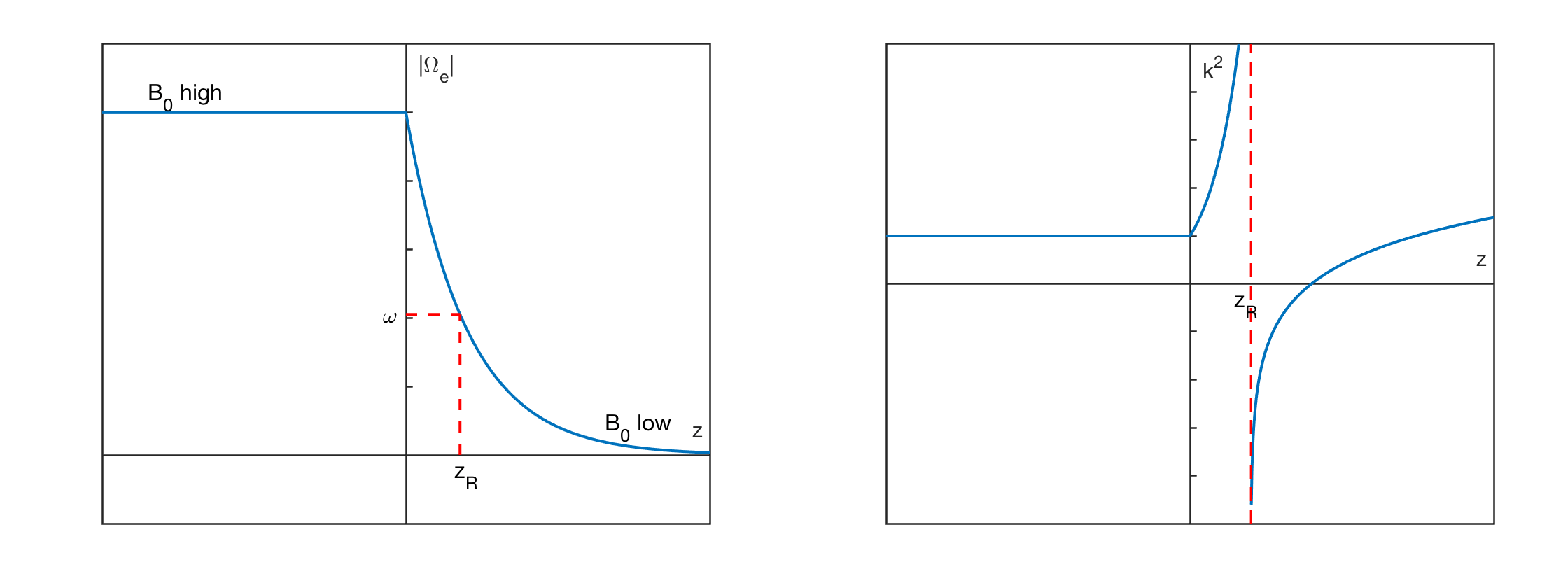
We use \(z\) here to remind ourselves of the fact that the wave property changes along the field line. Imagine a wave \(\sim e^{i(kz -\omega t)}\) incident into a plasma with fixed density \(n_0\) and varying magnetic field \(B_0(z)\) as shown in Figure 7.9(a). At \(z=z_R\), \(\omega_{ce}(z) = \omega_{ce}(z_R) = \omega\). Then we can draw \(k^2(z)\) as a function of \(z\) as in Figure 7.9(b). There is a pole at \(z=z_R\), which indicates resonance since \(k^2\rightarrow\infty\). There is also a zero on the right of \(z_R\).

Close to \(z=z_R\), we have \(k^2(z)\sim \frac{\text{const}.}{z-z_R}\). If we write \[ \Omega_e(z)=-A^\prime (z-z_R)+\omega,\quad \zeta = z-z_R \]

then (ignore the constants) \[ \frac{\mathrm{d}^2 E}{\mathrm{d}z^2} - \frac{\text{const.}}{z-z_R}E = 0 \Rightarrow \frac{\mathrm{d}^2 E}{d\zeta^2} - \frac{1}{\zeta}E = 0 \]

Now let’s stare at Figure 7.9(b) for a few seconds. If there is a wave from left to right, there will be a resonance at \(z=z_R\); but if there is a wave from right to left, then the wave will be attenuated before it reaches \(z=z_R\) because there is a zero ahead. This means that waves from different origin will have different behaviors!

7.12.3 O-mode

Next consider EM waves in non-magnetized plasma of ordinary O-mode: \[ k^2(x) = \frac{\omega^2}{c^2}n^2 = \frac{\omega^2}{c^2}\Big[ 1-\frac{{\omega_{pe}(x)}^2}{\omega^2}\Big] \quad \text{if } n \text{ is non-uniform} \]

Figure 7.10: Plasma frequency and wave number as functions of \(x\) in a non-uniform plasma for O mode.

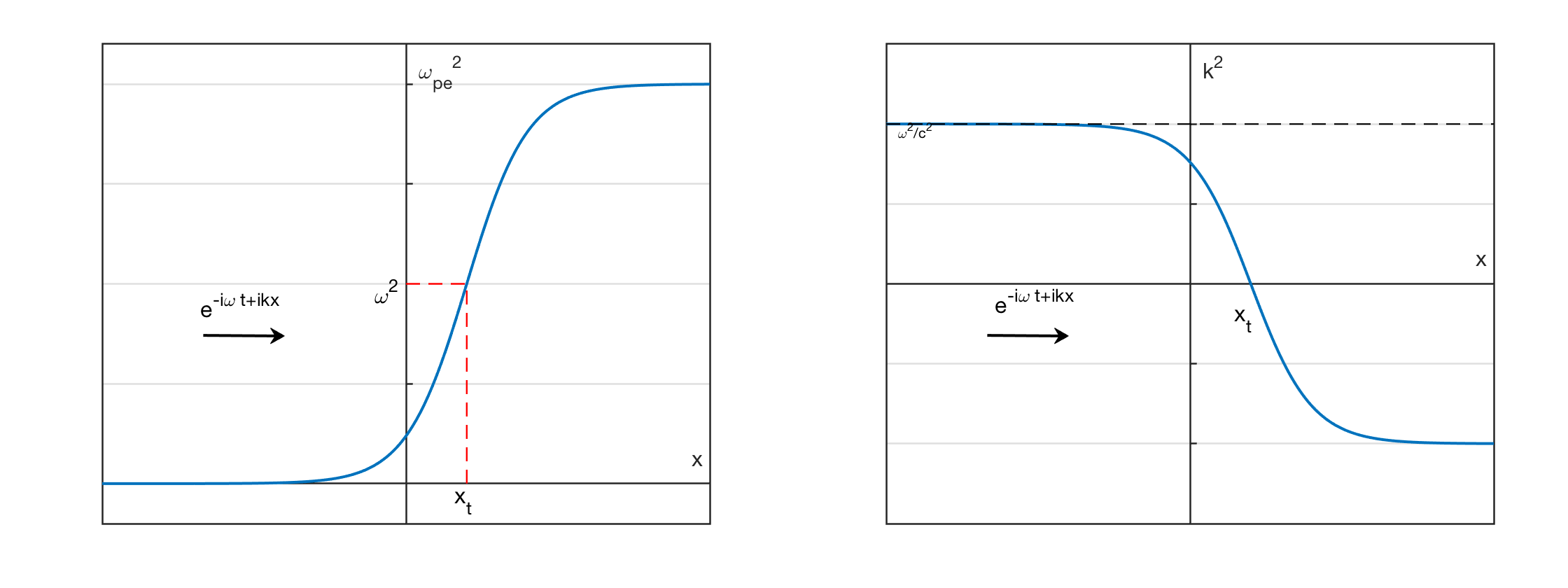
Note that there is no energy dissipation, because it is collisionless. Imagine a wave \(\sim e^{i(kx-\omega t)}\) incident into a plasma with density \(n_0(x)\) shown in Figure 7.10. We encounter a cutoff at \(x=x_t\), \(\omega_{pe}(x_t) = \omega\). Therefore we can draw \(k^2(x)\) as a function of x as in Figure 7.10. Then the properties of the wave can be categorized into two regimes: \[ \begin{aligned} k^2 < 0 \Rightarrow\ E\sim e^{\pm ikx}\ \text{propagating}\\ k^2 > 0 \Rightarrow\ E\sim e^{\pm|k| x}\ \text{attenuating} \end{aligned} \]

A natural question comes up from this picture: how does the propagating wave transform into attentuating wave? Stokes solved this during his honey moon, which is now known as the Stokes phenomenon (Section 3.11.3).

7.13 Warm Uniform Plasma

The analysis of cold plasma waves, although very complicated already, leaves out all of the physics that relates to finite temperature effects. These effects may be included in varying degrees of approximation, and it is intructive to include at this stage only the simplest thermal correction terms through the inclusion of a finite pressure term. For the sake of simplicity, we only consider the 1D case. The approach is very similar to cold plasma situation, except that we have pressure included in the equation, and we also need to specify the relation of pressure and temperature through the equation of state.

7.13.1 Two-fluid approach

Equilibrium: \[ \begin{aligned} &m_i=\infty,\ T_i=0,\ v_{i,0}=0,\ n_{e0}=n_{i0}=n_0,\ E_0=0,\ B_0=0 \\ &P_0=const.,\ v_{e0}=0 \end{aligned} \]

The equation of motion for electron is \[ \frac{\partial \mathbf{v}}{\partial t}+\mathbf{v}\cdot\nabla\mathbf{v}=-\frac{e}{m_e}\mathbf{E}-\frac{\nabla P}{\rho} \]

Assume \[ \begin{aligned} &P=P_0 \Big( \frac{n}{n_0}\Big)^\gamma &\text{adiabatic}\\ &P=nk_B T_e &\text{isothermal}(\gamma=1) \end{aligned} \]

Define \(P_1=\Big( \partial P/\partial \rho\Big)\rho_1\equiv {v_{th}}^2\rho_1={v_{th}}^2 n_1 m=k_BTn_1\). Decompose the primitive variables into equilibrium and perturbation components:

\[ \begin{aligned} &n= n_0+n_1=n_0+\tilde{n}_1e^{-i\omega t+ikx} \\ &v=\cancel{v_0}+v_1=\tilde{v}_1 e^{-i\omega t+ikx} \\ &P=P_0+P_1=P_0+\tilde{P}_1e^{-i\omega t+ikx} \end{aligned} \]

Substituting into the equation of motion and keeping only first order terms, we get \[ \begin{aligned} \frac{\partial v_1}{\partial t}&=-\frac{e}{m_e}(E_1)-\frac{\nabla (P_1)}{n_0m_e} \\ -i\omega v_1&=-\frac{e}{m_e}E_1-\frac{ik{v_{th}}^2 n_1}{n_0} \end{aligned} \]

The continuity equation gives \[ \begin{aligned} \frac{\partial n}{\partial t}+\frac{\partial}{\partial x}\Big( nv\Big)=0 \\ \Rightarrow v_1=\frac{\omega n_1}{kn_0} \end{aligned} \]

Substituting this into the linearized equation of motion, we get \[ n_1=\frac{kn_0eE_1}{im_e(\omega^2-k^2{v_{th}}^2)} \]

which is the density perturbation in response to \(E_1\). Following the same approach as before, we can easily get the dielectric function: \[ \frac{\epsilon}{\epsilon_0}=1-\frac{{\omega_{pe}}^2}{\omega^2-k^2{v_{th}}^2} \]

Let \(\epsilon=0\), we get the dispersion relation for warm plasma \[ \omega^2=k^2{v_{th}}^2+{\omega_{pe}}^2 \]

This is called the Bohm-Gross dispersion relation (BGDR). (Swanson 2012) has shown that by keeping higher order terms, \[ \omega^2 = \omega_{pe}^2\left[ 1 + \frac{3}{2}\left( \frac{k v_{th}}{\omega_{pe}} \right)^2 + \frac{15}{4}\left( \frac{k v_{th}}{\omega_{pe}} \right)^4 \right] \] so it is apparent that the moment expansion is an expansion in the ratio of the thermal velocity to the phase velocity. The BGDR now resolves the ambiguity in cold plasma theory and supports the notion that \(P=0\) in cold plasma is a cutoff rather than a resonance, since this dispersion relation describes a wave with a cutoff at \(\omega_{pe}\) that propagates near the electron thermal speed for high frequencies.

We see from this example that the fluid equations which are based on moment expansions are valid as long as the phase velocity is large compared to the thermal speed, \(v_p\gg v_{th}\).

7.13.2 Vlasov approach

Assume Maxwellian distribution for electrons: \[ g_e(v)=\frac{1}{\sqrt{2\pi}}\frac{1}{v_{th,e}}e^{-v^2/2{v_{th,e}}^2} \]

Assuming \(\frac{\omega}{k}\gg v_{th,e}\), i.e. the phase speed is much larger than the characteristic thermal speed, we can do Taylor series expansion \[ \frac{1}{(v-\omega/k)^2}=\frac{1}{(\omega/k)^2}\frac{1}{(1-kv/\omega)^2}\approx \frac{k^2}{\omega^2}\Big[ 1+\frac{2kv}{\omega}+\frac{3k^2v^2}{\omega^2}+...\Big] \]

Then the dielectric function is \[ \begin{aligned} \frac{\epsilon}{\epsilon_0}&=1-\frac{{\omega_{pe}}^2}{k^2}\int_{-\infty}^{\infty}dv g(v)\frac{k^2}{\omega^2}\Big[ 1+\frac{2kv}{\omega}+\frac{3k^2v^2}{\omega^2}+...\Big] \\ &\doteq 1-\frac{{\omega_{pe}}^2}{\omega^2}\Big[ 1+\frac{3k^2{v_{th}}^2}{\omega^2} \Big] . \end{aligned} \]

Let \(\epsilon=0\), we can get the dispersion relation for warm plasma, \[ \begin{aligned} &\text{lowest order: } \omega=\pm \omega_{pe} \\ &\text{first order:} 1-\frac{{\omega_{pe}}^2}{\omega^2}\Big( 1+\frac{3k^2{v_{th}}^2}{{\omega_{pe}}^2}\Big)=0\Rightarrow \omega^2={\omega_{pe}}^2+3k^2{v_{th,e}}^2 \end{aligned} \]

Note here we insert \(0^{th}\) order solution to \(1^{st}\) order equation to get the next level approximation. Comparing with the results from 2-fluid theory, we see that the expression is very similar except a discrepancy in the coefficient. This is owing to the fact that we do not specify \(\gamma\) in the equation of state. Actually, there are still ambiguities and debates about the exact equation of state. I wonder if I can get the exact coefficient under some assumption.

The opposite limit case: \(\frac{\omega}{k}\ll v_{th}\). From 2-fluid theory, \[ \frac{\epsilon}{\epsilon_0}\approxeq1+\frac{{\omega_{pe}}^2}{k^2{v_{th,e}}^2} \]

From Vlasov theory, \[ \begin{aligned} \frac{\epsilon}{\epsilon_0}&=1-\frac{{\omega_{pe}}^2}{k^2}\int_{-\infty}^{\infty}dv\frac{\partial g/\partial v}{v-\omega/k}= 1-\frac{{\omega_{pe}}^2}{k^2}\int_{-\infty}^{\infty}\frac{1}{v-\cancel{\omega/k}}\frac{1}{\sqrt{2\pi}}\frac{1}{v_{th,e}}\Big(\frac{-v}{{v_{th,e}}^2} \Big) e^{-v^2/2{v_{th,e}}^2}dv \\ &=1+\frac{{\omega_{pe}}^2}{k^2}\int_{-\infty}^{\infty}\frac{1}{v_{th,e}^2}\frac{1}{\sqrt{2\pi}} e^{-v^2/2{v_{th,e}}^2}dv \\ &=1+\frac{{\omega_{pe}}^2}{k^2{v_{th,e}}^2} \end{aligned} \]

So we can see in the two limit cases that they “almost” give the same results!

If we include ion motion in the 2-fluid theory (\(n_{1i}\neq0, T_i\neq0,m_i\neq\infty\)), applying the linear superposition property, we have

\[ \frac{\epsilon}{\epsilon_0}=\underbrace{1}_{\nabla\cdot(\epsilon_0\mathbf{E}_1)}-\underbrace{\frac{{\omega_{pe}}^2}{\omega^2-k^2{v_{th,e}}^2}}_{en_{1e}}-\underbrace{\frac{{\omega_{pi}}^2}{\omega^2-k^2{v_{th,i}}^2}}_{en_{1i}} \]

7.13.3 Ion-acoustic wave

Assume \(v_{th,e}\gg \frac{\omega}{k}\gg v_{th,i}\), we have the simplified dielectric function \[ \frac{\epsilon}{\epsilon_0}=1+\frac{{\omega_{pe}}^2}{k^2{v_{th,e}}^2}-\frac{{\omega_{pi}}^2}{\omega^2} \]

Assume quasi-neutrality condition: \(n_{1e}\approx n_{1i}\), s.t. \[ \nabla\cdot(\epsilon_0\mathbf{E}_1)=e(n_{1e}-n_{1i})\approx 0 \] so we can ignore the “1” in the dielectric function. Let \(\epsilon=0\), we get \[ \begin{aligned} \frac{{\omega_{pe}}^2}{k^2{v_{th,e}}^2}-\frac{{\omega_{pi}}^2}{\omega^2}=0 \\ \Rightarrow \omega^2=k^2{v_{th,e}}^2\frac{m_e}{m_i},\ \frac{\omega}{k}=\sqrt{\frac{k_BT_e}{m_i}}\equiv c_s \end{aligned} \]

Physically, electron sees the electric field created by ions due to ion plasma oscillation. Since electrons move much faster than ions, this electric field is nearly electrostatic for electrons. As a result, electron just follows the ion motion.

There are some other ways to get the ion-acoustic wave. If \(\omega\ll \omega_{pe}\), we can treat this wave as electrostatic wave for electron. The distribution for electron number density is \[ \begin{aligned} &n_{e}=n_0e^{e\phi/k_B T_e}\approxeq n_{0e}+n_{1e} \approxeq n_0[1+\frac{e\phi}{k_BT_e}+...] \\ \Rightarrow &n_{1e}=n_0\frac{e\phi}{k_BT_e}=\frac{n_0eE_1}{-ikm_e{v_{th,e}}^2} \end{aligned} \]

Note that here the tilde signs \(\sim\) of the variables are neglected for convenience without ambiguity.

Do we need to calculate \(n_{1i}\)??? Yes. MORE to do here!

Also, from the linearized equation of motion for electron, \[ \begin{aligned} \frac{\partial v_{e1}}{\partial t}=-\frac{e}{m_e}E_1-\frac{\nabla P_1}{n_0m_e} \\ -i\omega v_{e1}=-\frac{e}{m_e}E_1-\frac{ik P_1}{n_0m_e}=-\frac{e}{m_e}E_1-\frac{ik n_{1e}k_BT_e}{n_0m_e} \end{aligned} \]

In the \(\omega\rightarrow 0\) limit, \(LHS\doteq0\), we get \[ n_{1e}= \frac{n_0eE_1}{-ikm_e{v_{th,e}}^2} \]

Then again we get the dielectric function through Poisson’s equation.

7.14 Electrostatic Wave in a Magnetized Plasma

Now we continue to discuss the property of electrostatic waves with background magnetic field.

First let us introduce a useful result for continuity equation. Assuming \(n_0=n_0(\mathbf{x}),\ \mathbf{v}_0=\mathbf{v}_0(\mathbf{x})\) in equilibrium, \(\mathbf{x}_1=\mathbf{x}_1(\mathbf{x},t)\) is the perturbation in displacement. We can show that the linearized continuity equation has an equivalent form: \[ \frac{\partial n_1(\mathbf{x},t)}{\partial t}+\nabla\cdot[ n_0(\mathbf{x})\mathbf{v}_1(\mathbf{x},t)+n_1(\mathbf{x},t)\mathbf{v}_0(\mathbf{x},t)]=0 \Leftrightarrow n_1(\mathbf{x},t)=-\nabla\cdot[n_0(\mathbf{x})\mathbf{x}_1(\mathbf{x},t)] \]

The proof is related to mass conservation shown as follows. Intuitively, you can think of this as the degree of condensation only depends on displacement, not on how you get there (speed).

In 1D, \[ \begin{aligned} n_0=n_0(x_0)=\text{unperturbed density} \\ x= x_0+x_1(x_0,t)=\text{instantanenous position} \\ n(x_0,t)=n_0(x_0)+n_1(x_0,t)=\text{total density} \end{aligned} \]

At time \(t\), \([x_0,x_0+\mathrm{d}x]\rightarrow[x_0+x_1(x_0,t),x_0+\mathrm{d}x+x_1(x_0+\mathrm{d}x,t)]\). Due to mass conservation, we have (This looks like the derivation of deformation in fluid dynamics.)

\[ \begin{aligned} n_0(x_0)\mathrm{d}x&=[n_0(x_0+x_1)+n_1(x_0+x_1,t)]\cdot[x_0+\mathrm{d}x+x_1(x_0+\mathrm{d}x,t)-(x_0+x_1(x_0,t))] \\ &\approx \Big[n_0(x_0)+x_1\frac{\partial n_0(x_0)}{\partial x_0}+n_1(x_0,t)\Big]\mathrm{d}x\Big[1+\frac{\partial x_1(x_0,t)}{\partial x_0}\Big] \end{aligned} \]

\[ \begin{aligned} &\Rightarrow n_0(x_0)=n_0(x_0)+n_0(x_0)\frac{\partial x_1(x_0,t)}{\partial x_0}+x_1\frac{\partial n_0(x_0)}{\partial x_0}+n_1(x_0,t) \\ &\Rightarrow n_1(x_0,t)=-n_0(x_0)\frac{\partial x_1(x_0,t)}{\partial x_0}-x_1\frac{\partial n_0}{\partial x_0}=-\frac{\partial}{\partial x_0}\big[ n_0(x_0)x_1(x_0,t) \big] \\ &\Rightarrow n_1(x,t)=-\frac{\partial}{\partial x}\big[ n_0(x)x_1(x,t)\big] \end{aligned} \]

The simplest equilibrium state in a constant magnetized plasma is \[ \begin{aligned} &n_{i0}=n_{e0}=n_0,\ \mathbf{E}_0=0,\ \mathbf{B}_0=B_0\widehat{z} \\ &\mathbf{v}_{e0}=\mathbf{v}_{i0}=0,\ T_e=0,\ T_i=0,\ m_i=\infty \end{aligned} \]

Now introduce an electrostatic perturbation (\(\mathbf{E}_1=-\nabla\phi_1\)) \[ \begin{aligned} \mathbf{E}_1=\tilde{\mathbf{E}_1}e^{-i\omega t+i\mathbf{k}\cdot\mathbf{x}}=-i\mathbf{k}\tilde{\phi}_1 e^{-i\omega t+i\mathbf{k}\cdot\mathbf{x}} \end{aligned} \]

we can confirm that this is indeed an electrostatic perturbation since \(\mathbf{E}_1\parallel \mathbf{k}\) and \(\mathbf{B}_1=0\).

Case 1: \(\mathbf{k}=k_z\widehat{z}\parallel \mathbf{B}_0\), i.e. parallel propagation. Then \(\mathbf{E}_1=\widehat{z}E_{1z}e^{-i\omega t+ik_z z}\). This is the same as if there is no magnetic field, so the dielectric function is

\[ \frac{\epsilon}{\epsilon_0}=1-\frac{{\omega_{pe}}^2}{\omega^2} \]

Case 2: \(\mathbf{k}\perp \mathbf{B}_0\), i.e. perpendicular propagation. Without loss of generality, let \(\mathbf{k}=k_x\widehat{x}\). Then

\[ \mathbf{E}_1=\widehat{x}\tilde{E}_{1x}e^{-i\omega t+ik_x x} \]

The equations of motion (cold plasma) in the \(x\) and \(y\) direction are \[ \begin{aligned} \ddot{x}_1 &= -\frac{e}{m_e}[E_{1x}+\dot{y}_1B_0] \\ \ddot{y}_1 &= -\frac{e}{m_e}[-\dot{x}_1B_0] \\ \Rightarrow \dot{y}_1&=\frac{eB_0}{m_e}x_1=|\Omega_e| x_1 \\ \ddot{x}_1&=-\frac{e}{m_e}[E_{1x}+|\Omega_e|\cdot{y_1}B_0]=-\frac{e}{m_e}E_{1x}-{\Omega_e}^2 x_1, \\ \Rightarrow x_1&=\frac{-\frac{e}{m_e}E_{1x}}{-\omega^2+{\Omega_e}^2} \end{aligned} \]

Then we have the perturbed density in response to the perturbed electric field \(E_{1x}\): \[ \begin{aligned} n_1=-n_0\nabla\cdot\mathbf{x}_1=-n_0ik_x x_1=-n_0ik_x\frac{-\frac{e}{m_e}E_{1x}}{-\omega^2+{\Omega_e}^2} \end{aligned} \]

From Poisson’s equation, we get the dielectric function (the same method as before): \[ \frac{\epsilon}{\epsilon_0}=1-\frac{{\omega_{pe}}^2}{\omega^2-{\Omega_e}^2} \]

Let \(\epsilon=0\), we have \[ \omega=\sqrt{{\omega_{pe}}^2+{\Omega_e}^2}\equiv \omega_{UH} \] which is called the upper hybrid frequency. This is the highest characteristic frequency in plasma. This upper hybrid wave is a havoc to some beam generator devices as it appears near the electron collector.

What if ions are included? Similar to previous derivations and notice that we are still within the range of linear theory, we have \[ \frac{\epsilon}{\epsilon_0}=1-\frac{{\omega_{pe}}^2}{\omega^2-{\Omega_e}^2}-\frac{{\omega_{pi}}^2}{\omega^2-{\Omega_i}^2} \]

For \(\Omega_i\ll \omega\ll \Omega_e\) with quasi-neutrality condition \(n_{1e}\approx n_{1i}\), we can have a simplified dispersion relation by letting \(\epsilon=0\): \[ \begin{aligned} &\frac{{\omega_{pe}}^2}{{\Omega_{e}}^2}=\frac{{\omega_{pi}}^2}{\omega^2}\\ \Rightarrow& \omega=\sqrt{{\omega_{pi}}^2\frac{{\Omega_e}^2}{{\omega_{pe}}^2}}=\sqrt{|\Omega_e \Omega_i|}\equiv \omega_{LH} \end{aligned} \] which gives us the low hybrid wave frequency. It equals to the geometric mean of the two cyclotron frequencies. Actually, this can be obtained from pure plasma motion argument. Recall that \(\Omega_i \ll \omega \ll \Omega_e\) means that for electrons the plasma seems to be nonmagnetized, so they moves only under the electric field, \[ v_{1ex}=\frac{-eE_{1x}}{m_e(-i\omega)} \]

On the other hand, for ions the magnetic field is strong while electric field still exists, so it experiences polarization drift along the direction of perturbed electric field, \[ v_{1ix}=\frac{1}{\Omega_i}\frac{\partial}{\partial t}\Big( \frac{E_{1x}}{B_0}\Big) \]

Under quasi-neutrality condition, \(v_{1ix}=v_{1ex}\), so we have \[ \frac{-eE_{1x}}{m_e(-i\omega)}=\frac{1}{\Omega_i}\frac{\partial}{\partial t}\Big( \frac{E_{1x}}{B_0}\Big) \Rightarrow \omega=\sqrt{|\Omega_e \Omega_i|} \]

If we consider warm plasma for 1D, there is an additional pressure term in the momentum equation. The continuity equation together with Poisson’s equation give the relation of perturbed displacement and electric field: \[ \begin{aligned} &n_1=-\nabla\cdot(n_0\mathbf{x}_1)=-ik_xn_0x_1 \\ &\nabla\cdot(\epsilon_0\mathbf{E}_1)=ik_x\epsilon_0E_{1}=-en_{1e}=eik_xn_0x_1 \\ \Rightarrow& E_{1}=\frac{en_0x_1}{\epsilon_0} \end{aligned} \]

Substituting into the momentum equation, we get \[ \begin{aligned} \ddot{x}_1+{\Omega_e}^2x_1&=-\frac{e}{m_e}E_{1}-\frac{\nabla P_1}{n_0m_e} \\ &=-{\omega_{pe}}^2 x_1-{k_x}^2{v_{th,e}}^2x_1 \end{aligned} \] where \(v_{th,e}=\sqrt{k_BT_e/m_e}\). This gives us (You can gain a sense of the equivalent force law from the dispersion relation.) \[ \omega^2={\omega_{pe}}^2+{\Omega_e}^2+{k_x}^2{v_{th,e}}^2 \]

This is also equivalent to the dielectric function \[ \frac{\epsilon}{\epsilon_0}=1-\frac{{\omega_{pe}}^2}{\omega^2-{\Omega_{e}}^2-{k_x}^2{v_{th,e}}^2} \]

7.15 CMA Diagram

The Clemmow-Mullaly-Allis (CMA) diagram classifies all EM + ES waves (including ions) in a cold magnetized plasma. However it is no longer useful in hot plasma waves.

• Resonances and cutoffs
• Mode conversions

7.16 Wave-Particle Interactions

Different wavemodes exchange energy with particles by different mechanisms including

1. Landau resonance which heats in the direction parallel to the magnetic field and can give a parallel beam in the velocity distribution function (VDF) (Figure 7.11 left). Charged particles exchange energy with \(E_\parallel\).

2. Cyclotron resonance which heats in the direction perpendicular to the magnetic field and broadens the velocity distribution function in the perpendicular direction (Figure 7.11 middle). Charged particles exchange energy with \(E_\perp\). Left-hand polarized ion cyclotron waves can lead to ion heating in the perpendicular direction.

3. Pitch angle scattering which can lead to the formation of a plateau in the VDF (Figure 7.11 right).

The resonance parameters for the Landau and cyclotron resonances are \[ \xi_\text{L} = \frac{\omega}{k_\parallel v_{\text{th},s}} \tag{7.92}\]

\[ \xi_\text{C} = \frac{\omega-\Omega_s}{k_\parallel v_{\text{th},s}} \tag{7.93}\]

Here the frequency \(\omega\) is measured in the plasma rest frame. \(\Omega_s\) denotes the cyclotron frequency of particle species \(s\) (ion species and electrons), \(k_\parallel\) the parallel component of the wavevector, and \(v_{\text{th},s}\) the particle thermal speed of species \(s\). In general, the resonance parameter can be defined for arbitrary harmonics of the cyclotron frequency \(m=0,\pm 1,\pm 2,...\): \[ \xi^{(m)} = \frac{\omega - m\Omega_s}{k_\parallel v_{\text{th},s}} \tag{7.94}\]

Figure 7.11: Wave-particle interactions and the associated part of the velocity distribution functions. Courtesy of Yasuhito Narita.

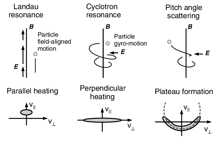
Note that the resonance parameters above are defined for a Maxwellian plasma. A correction is needed when treating a non-Maxwellian plasma to find the suitable velocity-space gradient for the resonance. The resonance is efficient when the parameter \(\xi_\text{L}\) or \(\xi_\text{C}\) is on the order of unity. Strictly speaking, the wave damping (or particle acceleration) is most efficient, typically for \(1<\xi<5\). The upper limit is not exact, but the resonance becomes gradually inefficient at larger values of \(\xi\). For \(\xi<1\) the particle motion is slower than the wave propagation and the particles do not have a sufficient time for exchanging energy with the wave electric field. For \(\xi>5\) there are increasingly fewer particles with higher velocities for the resonance (higher than the thermal speed).

7.16.1 Pitch Angle Scattering

Charged particles can be scattered by the wave electric and magnetic fields incoherently, and the scattering deforms the velocity distribution function along the co-centric contours centered at the wave phase speed (Figure 7.11, right panel). The reason for the deformation is that the particle kinetic energy \(K_{wv}\) (per unit mass) does not change in the co-moving frame with the apparent wave phase speed in the parallel direction to the mean magnetic field: \[ K_{wv} = \frac{1}{2}\left[ v_\perp^2 + \left( v_\parallel - \frac{\omega}{k_\parallel} \right)^2 \right] = \text{const}. \]

The co-centric deformation of the distribution function achieves a quasi-linear equilibrium in that the velocity–space gradient becomes zero (plateau formation) in the pitch angle directions. For example, in the solar wind ions are found to be resonating with obliquely propagating Alfvén/ion cyclotron waves. Note that the relevant phase speed is \(\omega/k_\parallel\), and is different from the true phase speed \(\omega/k\). The perpendicular component of the wavevector \(k_\perp\) does not play a role in pitch angle scattering.

This process is well explained by Plasma Zoo: Gyroresonant Scattering.

7.17 Whistler Wave

There exist different terminologies for whistler waves in the space and laboratory communities. In space science, a “whistle” is specifically defined as an electromagnetic wave excited by lightning and dispersed while propagating through the ionosphere and magnetosphere. All other excitation mechanisms lead to whistler-mode wave. Depending on their sound and spectrograms they are given many exotic names such as hiss, roar, saucers, chorus, risers, hooks, triggered emissions, etc, which are essentially the same thing with slightly different behaviors. In laboratory plasma physics any wave propagating in the whistler mode is simply called a whistler wave. However, in bounded laboratory plasmas, in particular solid state plasmas, these waves are often called helicons.

Whistler waves are most often referring to electron whistler waves, also known as electron cyclotron waves. Electron whistler waves are VLF emissions observed in the frequency range between the lower hybrid resonance frequency \(\omega_\mathrm{LH}\) (Equation 7.28) and electron gyrofrequency \(\Omega_\mathrm{e} = eB/m_e\).³ They are a type of electron-scale plasma waves that contribute to electron scattering, acceleration, and energy transport.⁴ They are driven by the electron temperature anisotropy (\(T_{e\perp}/T_{e\parallel}>1\), and the parallel energy of the resonant electrons exceeds the magnetic energy per electron, \(\mathcal{E}_\parallel = \frac{1}{2}m_e v_\parallel^2 > B^2 / 2\mu_0 n_e\), just like EMIC waves are stimulated by the temperature anisotropy of the ions (Kennel and Petschek 1966).) or by electron beams or heat fluxes (Gary 1993), and shape the electron velocity distribution function through wave-particle interactions.⁵ (Ren+ 2020)

Whistler modes are dispersive waves (i.e., group and phase velocities are frequency-dependent), which can propagate oblique to the static magnetic field \(\mathbf{B}_0\) up to a limiting “resonance cone” angle, given for electrons by (Stenzel 1999) \[ \theta_{\mathrm{phase, max}} = \cos^{-1}(\omega/\Omega_e) \]

Near the oblique resonance the group and phase velocities are essentially orthogonal, and the wave energy is dominated by the electric field. For frequencies \(\omega < \Omega_e/2\) there exists an oblique mode at \(\theta_\mathrm{phase} = \cos^{-1}(2\omega/\Omega_e)\) with parallel group velocity called the Gendrin mode [Gendrin 1961]. Along the direction of wave propagation \(\mathbf{k}\) the wave magnetic field is right-hand circularly polarized. The electric field of oblique whistlers has both space charge and inductive contributions, \(\mathbf{E} = -\nabla \phi - \partial \mathbf{A}/\partial t\). At an oblique density discontinuity the reflection of whistlers produces two reflected and one transmitted mode [Lee, 1969]. Refraction of whistlers in density nonuniformities has been studied carefully [Smith, 1961; Helliwell, 1965; Walker, 1976] since it explains the remarkable ducting properties of whistlers. Ducting confines the wave energy in a field-aligned density crest or trough and allows oblique whistlers to propagate undamped over long distances along \(\mathbf{B}_0\). All ground observations of whistlers, in particular the multiply reflected whistlers, involve ducting.

Plane whistler waves can decay because of

• electron collisions with neutrals and ions,
• collisionless electron cyclotron damping (\(\omega - \Omega_e = \mathbf{k}\cdot\mathbf{v}_e\)), and
• Landau damping for oblique modes (\(\omega = \mathbf{k}\cdot\mathbf{v}_e\)).

and it can grow when the distribution function at the resonant velocity has a positive slope because of

• Cherenkov instabilities
• cyclotron resonance
• Landau resonance

Whistler wave can decay into lower hybrid and kinetic Alfven waves. Parametric instabilities can trap whistler decay waves along the resonance cone. The stability of whistlers in plasmas with non-Maxwellian distribution functions has been studied theoretically in detail [Lee and Crawford, 1970]. The interaction of Langmuir waves and whistlers can produce the observed filamentary fine structure of solar type IV radio bursts [Fomichev and Fainshtein, 1988].

Note that there are also MHD whistler modes in the range of the ion cyclotron frequency \(\Omega_i\) [Russell+ 1971; Albert, 1980]. Properties of whistler waves can relate closely to electron-scale physics in magnetic reconnection (e.g. (Wang et al. 2023) at Mars, THEMIS observation in Earth’s tail reconnection exhaust region, and lower-hybrid instability).

We first see the derivations of whistler wave dispersion relation in Section 7.7 at the low frequency MHD limit. Another way to derive the whistler mode dispersion relation, which is probably easier, is to include the Hall term from the generalized Ohm’s law: \[ \mathbf{E} = -\mathbf{U}\times\mathbf{B} + \frac{1}{ne}\mathbf{J}\times\mathbf{B} \]

Using Ampère’s law and retaining only the Hall term leads to the equation \[ \dot{\mathbf{B}} = -\frac{1}{\mu_0 ne}\nabla\times[(\nabla\times\mathbf{B})\times\mathbf{B}] \]

Performing linearization and assuming that the magnetic field is parallel to the z-axis and its perturbation is only in x and y, the last equation becomes \[ \begin{aligned} \omega B_{1x} &= -i\frac{k_z^2 B_0}{\mu_0 ne} B_{1y} \\ \omega B_{1y} &= i\frac{k_z^2 B_0}{\mu_0 ne} B_{1x} \end{aligned} \] which easily yields \[ \omega = \frac{B_0}{\mu_0 ne} k_z^2 \]

This is the \(v_A\ll W\) case in Equation 7.25 where \(v_w = W\). For a more complete derivation, see Chen Shi’s note. The dispersion relations of whistler and ion cyclotron wave make a pair, similar to the relation between fast and slow magnetosonic waves.

The dispersion property of whistler waves makes it a problem for hybrid simulations (Section 26.3).

Figure 7.12: Whistler wave.

In situ measurements are sensitive to the entire spectrum of oblique whistlers (\(\omega < \Omega_e \cos\theta\)), hence most of the observed whistlers are oblique, unducted, magnetospherically reflected waves (Stenzel 1999). ???

7.17.1 Ducting of Whistler Waves

Ducting refers to the confinement of whistler waves within channels or “ducts” formed by variations in plasma density along the magnetic field lines. The density can be modulated by instabilities and thereby modifies the whistler wave propagation and amplitude. Most common are density modifications via the ponderomotive force, thermal pressure, and ionization, which can lead to self-focusing and filamentation instabilities.

• Density Enhancements and Depletions: Whistler waves can become trapped within regions of higher or lower plasma density relative to the surrounding environment. These density variations create what are called ducts.

• Refraction: The speed of a whistler wave depends on the plasma density. As whistler waves encounter changes in density along a magnetic field line, they undergo refraction (bending), similar to how light bends when passing between different materials.

• Confinement: The refraction caused by density gradients can keep the whistler waves confined within the duct. The waves essentially bounce back and forth within the duct as they propagate along the magnetic field line.

Types of Ducts:

1. Density Enhancement Ducts: Whistler waves become trapped in regions of higher plasma density.
2. Density Depletion Ducts: Whistler waves become trapped in regions of lower plasma density.

Significance of Ducting:

• Wave Guidance: Ducting allows whistler waves to travel over much longer distances than they otherwise would in a homogeneous plasma.
• Wave Amplification: Ducting can lead to the amplification of whistler wave intensity.
• Interaction with Particles: Ducted whistler waves can interact with charged particles trapped in the Earth’s radiation belts, leading to particle acceleration, scattering, and loss. This plays a crucial role in the dynamics of the radiation belts.

7.17.2 Whistlers in EMHD

While many wave phenomena are thought of in terms of plane monochromatic eigenmodes, a vast class of whistler phenomena arise in the form of temporal transients and spatially bounded phenomena, i.e., wave packets. Such transient phenomena are common in electron magnetohydrodynamicss (EMHD) physics (Chapter 8). In contrast to ordinary MHD where the plasma behaves like a single magnetized fluid, in EMHD only the electrons are magnetized while the ions are not. This arises on timescales \(f_{ce}^{-1} < t < f_{ci}^{-1}\) and spatial scales \(r_{Le} < r < r_{Li}\). The transition region is the Hall MHD. Refer to Stenzel (1999) for more detailed comparisons.

Specifically for whistlers, the whistler wave can be described by EMHD on timescales of \(2\pi/\Omega_{ce}<t<2\pi/\Omega_{LH}\) and spatial scales of \(L<\lambda_i\), where the ions are assumed as a motionless neutralizing background [Zhao 2017]. When magnetic field lines are fully frozen into the electron fluid, the whistler wave follows the dispersion relation \(\omega=\Omega_{ce}\lambda_e^2 k^2\cos\theta\). The dispersion relation becomes \(\omega=\Omega_{ce}\lambda_e^2 k^2\cos\theta/(1+\lambda_e^2 k^2)\) as the electron inertia is contained in Ohm’s law. Jinsong Zhao further extended the model by taking the electron thermal pressure and the displacement current into the EMHD model.

7.17.3 Importance of whistler

1. They play an important role in both the acceleration and loss of electrons in the radiation belt in the inner magnetosphere (See the series of studies by Thorne, R. M).

Lower energy electrons (~ keV) generate chorus waves -> relax temperature anisotropy -> waves scatter electrons into the loss cone and lead to electron precipitation into the ionosphere.

2. Chorus wave is the driver of pulsating aurora (Nishimura+ 2010) and diffuse aurora (Thorne+ 2010).

3. Chorus waves may be the source of hiss waves in the plasmasphere. Hiss waves play an important role in scattering electrons into the loss cone in the slot region.

7.18 Wave Identification

Measured wave spectra are complex and opaque, i.e. it is very difficult from an inspection of their shape to identify the wave modes that are present in the plasma volume under investigation. In some rare clean cases one can conclude from the observation of a particular maximum peak in the wave power or the observation of only one single field component which wave has been detected. In the general case of broad spectra or mixed spectral peaks and various field components lacking clear dominance of one field component it becomes nearly impossible to decide about the waves. Clearly, when the spectrum is a shapeless power-law one, in most cases, we are dealing with developed turbulence or localised structures in which case it makes no sense to distinguish and search for single modes. Then one must seek shelter among the well developed methods of analysing turbulence.

On the other hand, if the spectra indicate the presence of single waves, one would like to have some quantities at hand which help identifying which modes one is dealing with. It would be helpful if one could measure simultaneously both, the wave frequency and the wave number spectra. This is possible, however, only with sophisticated multi-spacecraft constellations. And even then only in the rarest cases the determination of the dispersion relation from experiment will be possible.

In application of these theoretical arguments to real observations one therefore has defined some quantities, called “transport ratios”, which have turned out to be quite valuable in helping identifying some of the wave modes. Such transport ratios for electromagnetic waves have been given by (Gary 1993).

• Polarization

The polarization of a wave magnetic field with respect to wave number \(\mathbf{k}\) is given by \[ P = i b_s / b_A \] where \(b_s, b_A\) are the components of the magnetic fluctuation field \(\mathbf{b}\) in the direction \(\mathbf{S},\mathbf{A}\) of magnetosonic and Alfvén waves, respectively, i.e. the vector \(\mathbf{A}=\mathbf{k}\times\mathbf{B}_0\) is perpendicular to the wave vector and the ambient magnetic field, while the vector \(\mathbf{S}\) is perpendicular to \(\mathbf{k}\) (because of the vanishing divergence \(\nabla\cdot\mathbf{b} = \mathbf{k}\cdot\mathbf{b}=0\)) in the plane \((\mathbf{k},\mathbf{B}_0)\). The waves are more magnetosonic or more Alfvénic whether \(|P|>1\) \(|P|<1\), respectively. For \(\Re(P)>0 (<0)\) the waves are right-hand (left-hand) polarized.

• Compression

The magnetic compression of the wave measures the relative variation in the parallel magnetic fluctuation field \[ C_B = \langle b_\parallel^2 \rangle / \langle |\mathbf{b}|^2 \rangle \] where the fluctuations are taken at a given pair \((\omega,\mathbf{k})\). The angular brackets \(\left< ab \right>\) mean taking the real part of the correlation function of the two bracketed quantities.

• Parallel compressibility

This ratio together with the compression ratio provides a tool for estimating how compressive a wave is. It is defined for species \(s\) as \[ C_{\parallel s} = \frac{B_0^2}{\langle b_\parallel^2 \rangle} \frac{\langle b_\parallel \Delta n_s \rangle}{n_s B_0} \]

• Non-coplanarity ratio

This ratio measures the fluctuating field component out of the plane \((\mathbf{k},\mathbf{B}_0)\), and is given by \[ C_c = \langle b_A^2 \rangle / \langle |\mathbf{b}|^2 \rangle \]

• Alfvén ratio: the ratio of velocity to magnetic fluctuations

Defining \(\delta\mathbf{v}_A = \mathbf{b} / \sqrt{\mu_0 m_i n}\) (unit V/B), where \(n\) is the total plasma density, the Alfvén ratio is defined as \[ R_{As} = \langle |\delta\mathbf{v}_s|^2 \rangle / \langle |\delta\mathbf{v}_A|^2 \rangle \] where \(\delta \mathbf{v}_s\) is the flow velocity of species \(s\). An Alfvén wave has \(\delta \mathbf{v}_i = \pm \mathbf{v}_A \mathbf{b}/\mathbf{B}_0\), and its own Alfvén ratio is \(R_{Ai} = 1\). The Alfvén ratio thus measures the fraction of Alfvén waves contained in the near-zero frequency fluctuations.

In another form, it can be written as \[ R_A = \mu_0 n m_i \frac{|\delta v_i|^2}{|\delta\mathbf{B}|^2} \]

One property that differs significantly is the Alfvén ratio where velocity fluctuations dominate for the kinetic slow wave and magnetic fluctuations dominate for the KAW.

• Cross helicity

Helicity of a wave is another identifier of the wave mode, it is in particular useful for determining the direction of propagation of the wave by considering its sign. See Section 15.2.6

7.19 Animation of Waves

Visualization is the best way of understanding physics.

Figure 7.13: Lower hybrid wave.

Bellan, Paul M. 2008. Fundamentals of Plasma Physics. Cambridge University Press.

Chen, Francis F. 2016. Introduction to Plasma Physics and Controlled Fusion. Vol. 1. Springer.

Chen, Liu, Fulvio Zonca, and Yu Lin. 2021. “Physics of Kinetic Alfvén Waves: A Gyrokinetic Theory Approach.” Reviews of Modern Plasma Physics 5 (1): 1–37. https://doi.org/10.1007/s41614-020-00049-3.

Gary, S Peter. 1993. Theory of Space Plasma Microinstabilities. 7. Cambridge university press.

Gurram, Harsha, Jan Egedal, and W Daughton. 2021. “Shear Alfvén Waves Driven by Magnetic Reconnection as an Energy Source for the Aurora Borealis.” Geophysical Research Letters 48 (14): e2021GL094201. https://doi.org/10.1029/2021GL094201.

Kennel, Charles F, and HE Petschek. 1966. “Limit on Stably Trapped Particle Fluxes.” Journal of Geophysical Research 71 (1): 1–28. https://doi.org/10.1029/JZ071i001p00001.

Stenzel, RL. 1999. “Whistler Waves in Space and Laboratory Plasmas.” Journal of Geophysical Research: Space Physics 104 (A7): 14379–95. https://doi.org/10.1029/1998JA900120.

Swanson, Donald Gary. 2012. Plasma Waves. Elsevier.

Verscharen, Daniel, Christopher HK Chen, and Robert T Wicks. 2017. “On Kinetic Slow Modes, Fluid Slow Modes, and Pressure-Balanced Structures in the Solar Wind.” The Astrophysical Journal 840 (2): 106. https://doi.org/10.3847/1538-4357/aa6a56.

Wang, Jing, Jiang Yu, Aojun Ren, Zuzheng Chen, Xiaojun Xu, Jun Cui, and Jinbin Cao. 2023. “In Situ Observations of Whistler-Mode Waves in Magnetic Reconnection at Mars.” The Astrophysical Journal 944 (1): 85. https://doi.org/10.3847/1538-4357/acb152.

---

1. This is different from the definition in optics, which makes it easier to analyze the interaction with particles since the particle gyration handedness around the magnetic field is also defined in the same way.

2. HOW TO DERIVE THIS?

3. [Tsurutani and Smith, 1974] said most often they are with a minimum wave power at \(0.5 \Omega_\mathrm{e}\). Is is observation or theory?

4. From Equation 7.24 we see the contribution of electron physics in the dispersion relation.

5. The derivation for the instability criterion involves kinetic theory, similar to the discussion in Chapter 11.