12 Kinetic Theory
12.1 Phase Space
Consider a particle moving in a one-dimensional space and let the position of the particle be \(x = x(t)\) and the velocity of the particle be \(v = v(t)\). A way to visualize the \(x\) and \(v\) trajectories simultaneously is to plot these trajectories parametrically on a two-dimensional graph, where the horizontal coordinate is given by \(x(t)\) and the vertical coordinate is given by \(v(t)\). This x-v plane is called phase-space. The trajectory (or orbit) of several particles can be represented as a set of curves in phase-space. Examples of a few qualitatively different phase-space orbits are shown in Figure 12.1.
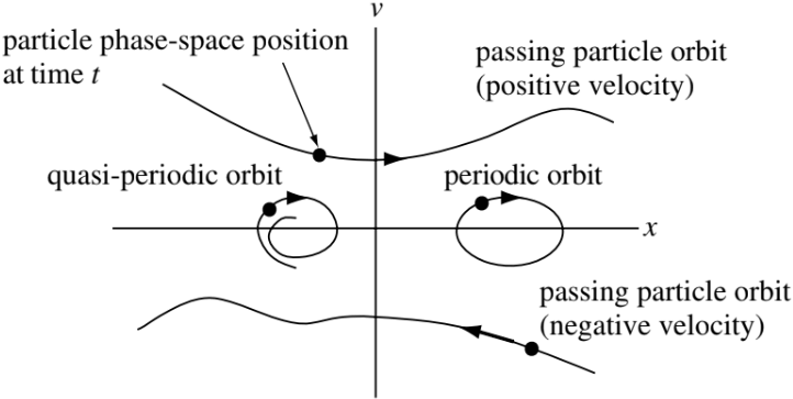
Particles in the upper half-plane always move to the right, since they have a positive velocity, while those in the lower half-plane always move to the left. Particles having exact periodic motion (e.g., \(x = A\cos t,\, v = −A\sin t\)) alternate between moving to the right and the left and so describe an ellipse in phase-space. Particles with quasi-periodic motions will have near-ellipses or spiral orbits. A particle that does not reverse direction is called a passing particle, while a particle confined to a certain region of phase-space (e.g., a particle with periodic motion) is called a trapped particle.
12.2 Distribution Function
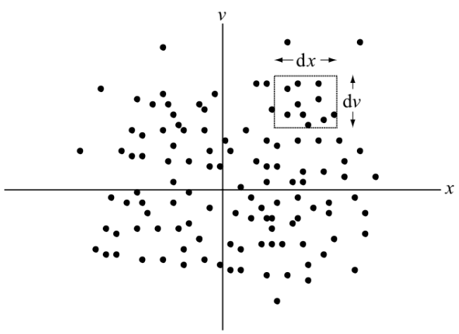
The fluid theory we have been using so far is the simplest description of a plasma; it is indeed fortunate that this approximation is sufficiently accurate to describe the majority of observed phenomena. There are some phenomena, however, for which a fluid treatment is inadequate. At any given time, each particle has a specific position and velocity. We can therefore characterize the instantaneous configuration of a large number of particles by specifying the density of particles at each point \(x, v\) in phase-space. The function prescribing the instantaneous density of particles in phase-space is called the distribution function and is denoted by \(f(x, v, t)\). Thus, \(f(x, v, t)\mathrm{d}x\mathrm{d}v\) is the number of particles at time \(t\) having positions in the range between \(x\) and \(x+\mathrm{d}x\) and velocities in the range between \(v\) and \(v+\mathrm{d}v\). As time progresses, the particle motion and acceleration causes the number of particles in these \(x\) and \(v\) ranges to change and so \(f\) will change. This temporal evolution of \(f\) gives a description of the system more detailed than a fluid description, but less detailed than following the trajectory of each individual particle. Using the evolution of \(f\) to characterize the system does not keep track of the trajectories of individual particles, but rather characterizes classes of particles having the same \(x, v\).
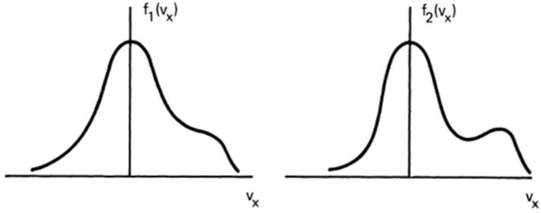
In fluid theory, the dependent variables are functions of only four independent variables: \(x, y, z,\) and \(t\). This is possible because the velocity distribution of each species is assumed to be Maxwellian everywhere and can therefore be uniquely specified by its bulk velocity \(\vec{U}\) and the temperature \(T\). Since collisions can be rare in high-temperature plasmas, deviations from thermal equilibrium can be maintained for relatively long times. As an example, consider two velocity distributions \(f_1(v_x)\) and \(f_2(v_x)\) in a one-dimensional system (Figure 12.2). These two distributions will have entirely different behaviors, but as long as the areas under the curves are the same, fluid theory does not distinguish between them.
When we consider velocity distributions in 3D, we have seven independent variables: \(f = f(\mathbf{r}, \mathbf{v}, t)\). By \(f(\mathbf{r}, \mathbf{v}, t)\), we mean that the number of particles per meter cubed at position \(\mathbf{r}\) and time \(t\) with velocity components between \(v_x\) and \(v_x + \mathrm{d}v_x\), \(v_y\) and \(v_y + \mathrm{d}v_y\), and \(v_z\) and \(v_z + \mathrm{d}v_z\) is \[ f(x, y, z, v_x, v_y, v_z, t) \mathrm{d}v_x \mathrm{d}v_y \mathrm{d}v_z \]
12.2.1 Moments of the distribution function
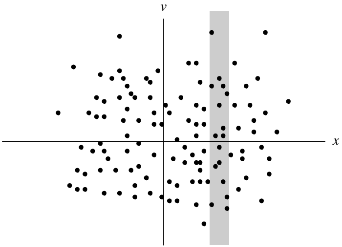
Let us count the particles in the shaded vertical strip in Figure 12.3. The number of particles in this strip is the number of particles lying between \(x\) and \(x + \mathrm{d}x\), where \(x\) is the location of the left-hand side of the strip and \(x + \mathrm{d}x\) is the location of the right-hand side. The number of particles in the strip is equivalently defined as \(n(x, t)\mathrm{d}x\), where \(n(x)\) is the density of particles at \(x\). Thus we see that \(\int f(x, v)\mathrm{d}v = n(x)\) the transition from a phase-space description (i.e., \(x, v\) are independent variables) to a conventional description (i.e., only \(x\) is an independent variable) involves “integrating out” the velocity dependence to obtain a quantity (e.g., density) depending only on position. Since the number of particles is finite, and since \(f\) is a positive quantity, \(f\) must vanish as \(v\rightarrow\pm\infty\).
In three-dimension, the density is now a function of four scalar variables, \(n=n(\mathbf{r}, t)\), which is the integral of the distribution function over the velocity space: \[ \begin{aligned} n(\mathbf{r}, t) &= \int_{-\infty}^{\infty} \mathrm{d}v_x \int_{-\infty}^{\infty} \mathrm{d}v_y \int_{-\infty}^{\infty} \mathrm{d}v_z f(\mathbf{r}, \mathbf{v}, t) \\ &= \int_{-\infty}^{\infty}f(\mathbf{r}, \mathbf{v}, t)\mathrm{d}^3v \\ &= \int_{-\infty}^{\infty}f(\mathbf{r}, \mathbf{v}, t)\mathrm{d}\mathbf{v} \end{aligned} \tag{12.1}\]
Note that \(\mathrm{d}\mathbf{v}\) is not a vector; it stands for a three-dimensional volume element in velocity space. If \(f\) is normalized so that \[ \int_{-\infty}^{\infty} \hat{f}(\mathbf{r}, \mathbf{v}, t) \mathrm{d}\mathbf{v} = 1 \tag{12.2}\]
Thus \[ \hat{f}(\mathbf{r}, \mathbf{v}, t) = f(\mathbf{r}, \mathbf{v}, t) / n(\mathbf{r}, t) \tag{12.3}\] is the probability that a randomly selected particle at position \(\mathbf{r}\) has the velocity \(\mathbf{v}\) at time \(t\). Using this point of view, we see that averaging over the velocities of all particles at \(x\) gives the mean velocity \[ u(\mathrm{x},t)=\frac{\int\mathbf{v}f(\mathbf{x},\mathbf{v},t)\mathrm{d}\mathbf{v}}{n(\mathbf{x},t)} \tag{12.4}\]
Similarly, multiplying \(\hat{f}\) by \(mv^2/2\) and integrating over velocity will give an expression for the mean kinetic energy of all the particles. This procedure of multiplying \(f\) by various powers of \(\mathbf{v}\) and then integrating over velocity is called taking moments of the distribution function.
Note that \(\hat{f}\) is still a function of seven variables, since the shape of the distribution, as well as the density, can change with space and time. From Equation 12.2, it is clear that \(\hat{f}\) has the dimensions \((\text{m}/\text{s})^{-3}\); and consequently, from Equation 12.3, \(f\) has the dimensions \(\text{s}^3 \text{m}^{-6}\).
12.2.2 Maxwellian Distribution
A particularly important distribution function is the Maxwellian: \[ \hat{f}_m = \left(\frac{m}{2\pi k_B T}\right)^{3/2}\exp\left(-\frac{v^2}{v_{th}^2}\right) \tag{12.5}\] where \[ v\equiv(v_x^2 + v_y^2 + v_z^2)^{1/2}\quad\text{and}\quad v_{th}\equiv(2k_B T/m)^{1/2} \]
This is the normalized form where \(\hat{f}_m\) is equivalent to probability: by using the definite integral \[ \int_{-\infty}^{\infty}\exp(-x^2)dx = \sqrt{\pi} \] one easily verifies that the integral of \(\hat{f}_m\) over \(\mathrm{d}v_x \mathrm{d}v_y \mathrm{d}v_z\) is unity.
A common question being asked is:
Why do we see Maxwellian/Gaussian/normal distribution ubiquitously in nature?
Well, this is related to the central limit theorem in statistics: in many situations, when independent random variables are summed up, their properly normalized sum tends toward a normal distribution even if the original variables themselves are not normally distributed (e.g. a biased coin which give 95% head and 5% tail). In statistical physics, this is related to the fact that a Maxwellian distribution represents the state of a system with the highest entropy under the constraint of energy conservation.
There are several average velocities of a Maxwellian distribution that are commonly used. The root-mean-square velocity is given by \[ (\overline{v^2})^{1/2} = (3k_B T/m)^{1/2} \]
The average magnitude of the velocity \(|v|\), or simply \(\bar{v}\), is found as follows: \[ \bar{v} = \int_{-\infty}^{\infty}v\hat{f}(\mathbf{v})d^3v \]
Since \(\hat{f}_m\) is isotropic, the integral is most easily done in spherical coordinates in v space. Since the volume element of each spherical shell is \(4\pi v^2 \mathrm{d}v\), we have \[ \begin{aligned} \bar{v} &= (m/2\pi k_B T)^{3/2}\int_0^\infty v[\exp(-v^2/v_{th}^2)]4\pi v^2 \mathrm{d}v \\ &= (\pi v_{th}^2)^{-3/2} 4\pi v_{th}^4 \int_0^\infty [\exp(-y^2)]y^3 dy \end{aligned} \]
The definite integral has a value 1/2, found by integration by parts. Thus \[ \bar{v} = 2\sqrt{\pi}v_{th} = 2(2k_B T/\pi m)^{1/2} \]
The velocity component in a single direction, say \(v_x\), has a different average. Of course, \(\bar{v}_x\) vanishes for an isotropic distribution; but \(|\bar{v}_x|\) does not: \[ |\bar{v}_x| = \int |v_x|\hat{f}_m(\mathbf{v})\mathrm{d}^3 v = \pi^{-1/2}v_{th} = (2k_B T/\pi m)^{1/2} \]
To summarize: for a Maxwellian, \[ \begin{aligned} v_{rms} &= (3k_B T/m)^{1/2} \\ |\bar{v}| &= 2(2k_B T/\pi m)^{1/2} \\ |\bar{v}_x| &= (2k_B T/\pi m)^{1/2} \\ \bar{v}_x &= 0 \end{aligned} \]
For an isotropic distribution like a Maxwellian, we can define another function \(g(v)\) which is a function of the scalar magnitude of \(\mathbf{v}\) such that \[ \int_0^\infty g(v) \mathrm{d}v = \int_{-\infty}^{\infty} f(\mathbf{v})\mathrm{d}v \]
For a Maxwellian, we see that \[ g(v) = 4\pi n (m/2\pi k_B T)^{3/2} v^2 \exp(-v^2/v_{th}^2) \tag{12.6}\]
(Add figure?) Note the difference between \(g(v)\) and a one-dimensional Maxwellian distribution \(f(v_x)\). Although \(f(v_x)\) is maximum for \(v_x=0\), \(g(v)\) is zero for \(v=0\). This is just a consequence of the vanishing of the volume in phase space for \(v=0\). Sometimes \(g(v)\) is carelessly denoted by \(f(v)\), as distinct from \(f(\mathbf{v})\); but \(g(v)\) is a different function of its argument than \(f(\mathbf{v})\) is of its argument. From Equation 12.6, it is clear that \(g(v)\) has dimensions \(\text{s}/\text{m}^4\).
(ADD EXAMPLE DISTRIBUTIONS!)
- Isotropic distribution
- Anisotropic (pancake) distribution
\[ f(v_\perp, v_\parallel) = \frac{n}{T_\perp T_\parallel^{1/2}}\Big( \frac{m}{2\pi k_B} \Big)^{3/2} \exp\Big( -\frac{mv_\perp^2}{2k_B T_\perp} - \frac{m(v_\parallel - v_{0\parallel})^2}{2k_B T_\parallel} \Big) \]
- Beam distribution
- Crescent shape distribution
It is often convenient to present the distribution function as a function of energy instead of velocity. If all energy is kinetic, the energy is simply obtained from \(W=mv^2/2\). In the case the particles are in the external electric potential field \(U=-q\varphi\) the total energy of particles is \(W=mv^2/2+U\) and the Maxwellian distribution is \[ f(v) = n\Big(\frac{m}{2\pi k_B T}\Big)^{3/2}\exp\Big(-\frac{W}{k_B T}\Big) \]
This can be written as the energy distribution (???): \[ g(W) = 4\pi\Big[ \frac{2(W-U)}{m^3} \Big]^{1/2} f(v) \]
The normalization factor is determined by requiring that the integration of the energy distribution over all energies gives the density.
Velocity and energy distribution functions cannot be measured directly. Instead, the observed quantity is the particle flux to the detector. Particle flux is defined as the number density of particles multiplied by the velocity component normal to the surface. We define the differential flux of particles traversing a unit area per unit time, unit solid angle (in spherical coordinates the differential solid angle is \(d\Omega = \sin\theta d\theta d\phi\)) and unit energy as \(J(W,\Omega, \alpha, \mathbf{r},t)\). (\(\alpha\) is species?) The units of \(J\) are normally given as \((\text{m}^2\text{sr}\,\text{s}\,\text{eV})^{-1}\).. Note that in literature \(\text{cm}\) is often used instead of \(\text{m}\) and, depending on the actual energy range considered, electron volts are often replaced by keV, MeV, or GeV.
Let us next define how differential particle flux and distribution function are related to each other. We can write the number density in a differential velocity element (in spherical coordinates \(\mathrm{d}^3v=v^2\mathrm{d}v\mathrm{d}\Omega\)) as (\(\mathrm{d}n=f(\alpha,\mathbf{r},t)v^2\mathrm{d}v\mathrm{d}\Omega\)). By multiplying this with \(v\) we obtain another expression for the differential flux \(f(\alpha,\mathbf{r},t)v^3dvd\Omega\). Comparing with our earlier definition of the differential flux we obtain \[ J(W,\Omega, \alpha, \mathbf{r},t)\mathrm{d}W\mathrm{d}\Omega = f(\alpha,\mathbf{r},t)v^3\mathrm{d}v\mathrm{d}\Omega \]
Since \(\mathrm{d}W=mv\mathrm{d}v\) we can write the relationship between the differential flux and the distribution function as \[ J(W,\Omega, \alpha, \mathbf{r},t) = \frac{v^2}{m}f \tag{12.7}\]
One application of the differential flux is the particle precipitation flux. With the idea of loss lone, we have a cone of particles that moves along the field lines and can propagate down to the ionosphere, and each shell from \(v\) to \(v+\mathrm{d}v\) corresponds to a specific energy range. This is something we can measure close to the ground and use to infer the plasma properties in the magnetosphere.
12.2.3 Kappa Distribution
The Maxwellian distribution is probably the most studied one theoretically, but may not be the most commonly observed distribution in a collisionless space plasma system. In recent years, another distribution named Kappa distribution has gained more attention.
Distribution functions are often nearly Maxwellian at low energies, but they decrease more slowly at high energies. At higher energies the distribution is described better by a power law than by an exponential decay of the Maxwell distribution. Such a behavior is not surprising if we remember that the Coulomb collision frequency decreases with increasing temperature as \(T^{-3/2}\) (Equation 9.23). Hence, it takes longer time for fast particles to reach Maxwellian distirbution than for slow particles. The kappa distribution has the form \[ f_\kappa(W) = n\Big( \frac{m}{2\pi\kappa W_0} \Big)^{3/2}\frac{\Gamma(\kappa + 1)}{\Gamma(\kappa-1/2)}\Big( 1+\frac{W}{\kappa W_0} \Big)^{-(\kappa+1)} \]
Here \(W_0\) is the energy at the peak of the particle flux and \(\Gamma\) is the gamma function. When \(\kappa\gg 1\) the kappa distribution approaches the Maxwellian distribution. When \(\kappa\) is smaller but \(>1\) the distribution has a high-energy tail. A thorough review is given by (Livadiotis and McComas 2013).
12.2.4 Entropy of a distribution
Collisions cause the distribution function to tend towards a simple final state characterized by having the maximum entropy for the given constraints (e.g. fixed total energy). To see this, we provide a brief discussion of entropy and show how it relates to a distribution function.
Suppose we throw two dice, labeled \(A\) and \(B\), and let \(R\) denote the result of a throw. Thus \(R\) ranges from 2 through 12. The complete set of (A,B) combinations that gives these \(R\)’s is listed in Table 12.1:
| \(R\) | \((A,B)\) |
|---|---|
| 2 | (1,1) |
| 3 | (1,2),(2,1) |
| 4 | (1,3),(2,2),(3,1) |
| 5 | (1,4),(2,3),(3,2),(4,1) |
| 6 | (1,5),(2,4),(3,3),(4,2),(5,1) |
| 7 | (1,6),(2,5),(3,4),(4,3),(5,2),(6,1) |
| 8 | (2,6),(3,5),(4,4),(5,3),(6,2) |
| 9 | (3,6),(4,5),(5,4),(6,3) |
| 10 | (4,6),(5,5),(6,4) |
| 11 | (5,6),(6,5) |
| 12 | (6,6) |
There are six \((A, B)\) pairs that give \(R = 7\), but only one pair for \(R = 2\) and only one pair for \(R = 12\). Thus, there are six microscopic states (distinct \((A, B)\) pairs) corresponding to \(R = 7\) but only one microscopic state corresponding to each of \(R = 2\) or \(R = 12\). Thus, we know more about the microscopic state of the system if \(R=2\) or \(R=12\) than if \(R=7\). We define the entropy \(S\) to be the natural logarithm of the number of microscopic states corresponding to a given macroscopic state. Thus, for the dice, the entropy would be the natural logarithm of the number of \((A, B)\) pairs that correspond to a given \(R\). The entropy for \(R = 2\) or \(R = 12\) would be zero since \(S = \ln(1) = 0\), while the entropy for \(R = 7\) would be \(S = \ln(6)\) since there were six different ways of obtaining \(R = 7\).
If the dice were to be thrown a statistically large number of times the most likely result for any throw is \(R = 7\) this is the macroscopic state with the largest number of microscopic states. Since any of the possible microscopic states is an equally likely outcome, the most likely macroscopic state after a large number of dice throws is the macroscopic state with the highest entropy.
Now consider a situation more closely related to the concept of a distribution function. In order to do this we first pose the following simple problem: suppose we have a pegboard with \(\mathcal{N}\) holes, labeled \(h_1\), \(h_2\), …, \(h_{\mathcal{N}}\) and we also have \(\mathcal{N}\) pegs labeled by \(p_1\), \(p_2\), …, \(p_{\mathcal{N}}\). What is the number of ways of putting all the pegs in all the holes? Starting with hole \(h_1\), we have a choice of \(\mathcal{N}\) different pegs, but when we get to hole \(h_2\) there are now only \(\mathcal{N}-1\) pegs remaining so that there are now only \(\mathcal{N}-1\) choices. Using this argument for subsequent holes, we see there are \(\mathcal{N}!\) ways of putting all the pegs in all the holes.
Let us complicate things further. Suppose that we arrange the holes in \(\mathcal{M}\) groups. Say group \(G_1\) has the first 10 holes, group \(G_2\) has the next 19 holes, group \(G_3\) has the next 4 holes and so on, up to group \(\mathcal{M}\). We will use \(f\) to denote the number holes in a group, thus \(f(1)=10\), \(f(2)=19\), \(f(3)=4\), etc. The number of ways arranging pegs within a group is just the factorial of the number of pegs in the group, e.g., the number of ways of arranging the pegs within group 1 is just 10! and so in general the number of ways of arranging the pegs in the jth group is \([f(j)]!\).
Let us denote \(C\) as the number of ways of putting all the pegs in all the groups without caring about the internal arrangement within groups. The number of ways of putting the pegs in all the groups caring about the internal arrangements in all the groups is \(C\times f(1)!\times f(2)\times f(3)!\times ... f(4)!\), but this is just the number of ways of putting all the pegs in all the holes, i.e., \[ C\times f(1)!\times f(2)\times f(3)!\times ... f(4)! = \mathcal{N}! \] or \[ C = \frac{\mathcal{N}!}{C\times f(1)!\times f(2)\times f(3)!\times ... f(4)!} \]
Now \(C\) is just the number of microscopic states corresponding to the macroscopic state of the prescribed grouping \(f(1) = 10\), \(f(2) = 19\), \(f(3) = 4\), etc. so the entropy is just \(S = \ln C\) or \[ \begin{aligned} S &= \ln\left( \frac{\mathcal{N}!}{C\times f(1)!\times f(2)\times f(3)!\times ... f(4)!} \right) \\ &= \ln\mathcal{N}! - \ln f(1)! - \ln f(2)! - ... - \ln f(\mathcal{M})! \end{aligned} \]
Stirling’s formula shows that the large-argument asymptotic limit of the factorial function is \[ \lim_{k\rightarrow\infty} \ln k! = k\ln k - k \]
Noting that \(f(1)+f(2)+...+f(\mathcal{M})=\mathcal{N}\), the entropy becomes \[ \begin{aligned} S &= \mathcal{N}\ln\mathcal{N} - f(1)\ln f(1) - f(2)\ln f(2) - ... - f(\mathcal{M})\ln f(\mathcal{M}) \\ &= \mathcal{N}\ln\mathcal{N} - \sum_{j=1}^{\mathcal{M}}\ln f(j) \end{aligned} \]
The constant \(\mathcal{N}\ln\mathcal{N}\) is often dropped, giving \[ S = -\sum_{j=1}^{\mathcal{M}} f(j)\ln f(j) \]
If \(j\) is made into a continuous variable, say \(j \rightarrow v\) so that \(f(v)\mathrm{d}v\) is the number of items in the group labeled by \(v\) then the entropy can be written as \[ S = -\int\mathrm{d}v f(v)\ln f(v) \]
By now, it is obvious that \(f\) could be the velocity distribution function, in which case \(f(v)\mathrm{d}v\) is just the number of particles in the group having velocity between \(v\) and \(v+\mathrm{d}v\). Since the peg groups correspond to different velocity range coordinates, having more dimensions just means having more groups and so for three dimensions the entropy generalizes to \[ S = -\int\mathrm{d}\mathbf{v} f(\mathbf{v})\ln f(\mathbf{v}) \]
If the distribution function depends on position as well, this corresponds to still more peg groups, and so a distribution function that depends on both velocity and position will have the entropy \[ S = -\int\mathrm{d}\mathbf{x}\int\mathrm{d}\mathbf{v} f(\mathbf{x},\mathbf{v})\ln f(\mathbf{x},\mathbf{v}) \tag{12.8}\]
12.2.5 Effect of collisions on entropy
The highest entropy state is the most likely state of the system because the highest entropy state has the highest number of microscopic states corresponding to the macroscopic state. Collisions (or other forms of randomization) will take some initial prescribed microscopic state and scramble the phase-space positions of the particles, thereby transforming the system to a different microscopic state. This new state could in principle be any microscopic state, but is most likely to be a member of the class of microscopic states belonging to the highest entropy macroscopic state. Thus, any randomization process such as collisions will cause the system to evolve towards the macroscopic state having the maximum entropy.
An important shortcoming of this argument is that it neglects any conservation relations that have to be satisfied. To see this, note that the expression for entropy could be maximized if all the particles are put in one group, in which case \(C = \mathcal{N}!\) which is the largest possible value for \(C\). Thus, the maximum entropy configuration of \(\mathcal{N}\) plasma particles corresponds to all the particles having the same velocity. However, this would assign a specific energy to the system, which would in general differ from the energy of the initial microstate. This maximum entropy state is therefore not accessible in isolated systems, because energy would not be conserved if the system changed from its initial microstate to the maximum entropy state.
Thus, a qualification must be added to the argument. Randomizing processes will scramble the system to attain the state of maximum entropy consistent with any constraints placed on the system. Examples of such constraints would be the requirements that the total system energy and the total number of particles must be conserved. We therefore reformulate the problem as: given an isolated system with \(\mathcal{N}\) particles in a fixed volume \(V\) and initial average energy per particle \(\left<E\right>\), what is the maximum entropy state consistent with conservation of energy and conservation of number of particles? This is a variational problem because the goal is to maximize \(S\) subject to the constraint that both \(\mathcal{N}\) and \(\mathcal{N}\left<E\right>\) are fixed. The method of Lagrange multipliers can then be used to take into account these constraints. Using this method the variational problem becomes \[ \delta S - \lambda_1\delta\mathcal{N} - \lambda_2\delta(\mathcal{N}\left<E\right>) = 0 \] where \(\lambda_1\) and \(\lambda_2\) are as-yet undetermined Lagrange multipliers. The number of particles is \[ \mathcal{N} = V\int f\mathrm{d}v \]
The energy of an individual particle is \(E = mv^2/2\), where \(v\) is the velocity measured in the rest frame of the center of mass of the entire collection of \(\mathcal{N}\) particles. Thus, the total kinetic energy of all the particles in this rest frame is \[ \mathcal{N}\left<E\right> = V\int\frac{mv^2}{2}f(v)\mathrm{d}v \] and so the variational problem becomes \[ \delta\int\mathrm{d}v\left( f\ln f - \lambda_1 Vf - \lambda_2 V\frac{mv^2}{2}f \right) = 0 \]
Incorporating the volume \(V\) into the Lagrange multipliers, and factoring out the coefficient \(\delta f\), this becomes \[ \int\mathrm{d}v \delta f \left( 1+\ln f - \lambda_1 - \lambda_2\frac{mv^2}{2} \right) = 0 \]
Since \(\delta f\) is arbitrary, the integrand must vanish, giving \[ \ln f = \lambda_2\frac{mv^2}{2} - \lambda_1 \] where the “1” has been incorporated into \(\lambda_1\).
The maximum entropy distribution function of an isolated, energy and particle conserving system is therefore \[ f = \lambda_1\exp\left( -\lambda_2 mv^2/2 \right) \] which is the Maxwellian distribution function. We will often assume that the plasma is locally Maxwellian so that \(\lambda_1 = \lambda_1(\mathbf{x},t), \lambda_2 = \lambda_2(\mathbf{x},t)\). We define the temperature to be \[ k_B T_s(\mathbf{x},t) = \frac{1}{\lambda_2(\mathbf{x},t)} \]
The normalization factor is set to be \[ \lambda_1(\mathbf{x},t) = n_s(\mathbf{x},t)\left( \frac{m_s}{2\pi k_B T_s(\mathbf{x},t)} \right)^{N/2} \] where \(N\) is the dimensionality (1, 2 or 3) so that \(\int f_s(\mathbf{x},\mathbf{v},t)\mathrm{d}^N\mathbf{v}=n_s(\mathbf{x},t)\). Because the kinetic energy of individual particles was defined in terms of velocities measured in the rest frame of the center of mass of the complete system of particles, if this center of mass is moving in the lab frame with a velocity \(\mathbf{u}_s\), then in the lab frame the Maxwellian will have the form \[ f_s(\mathbf{x},\mathbf{v},t) = n_s\left( \frac{m_s}{2\pi k_B T_s} \right)^{N/2} \exp\left( -\frac{m_s(\mathbf{v}-\mathbf{u}_s)^2}{2k_B T_s} \right) \tag{12.9}\]
Equation 12.9 is equivalent to Equation 12.5 times number density in 3D.
12.3 Equations of Kinetic Theory
12.3.1 Vlasov equation
Now consider the rate of change of the number of particles inside a small box in phase-space, such as is shown in Figure 12.4. Defining \(a(x, v, t)\) to be the acceleration of a particle, it is seen that the particle flux in the horizontal direction is \(fv\) and the particle flux in the vertical direction is \(fa\). Thus, the particle fluxes into the four sides of the box are:
- flux into left side of box is \(f(x, v, t)v\mathrm{d}v\)
- flux into right side of box is \(-f(x+\mathrm{d}x, v, t)v\mathrm{d}v\)
- flux into bottom of box is \(f(x, v, t)a(x, v, t)\mathrm{d}x\)
- flux into top of box is \(-f(x, v+dv, t)a(x, v+dv, t)dx\)
The number of particles in the box is \(f(x, v, t)\mathrm{d}x\mathrm{d}v\) so that the rate of change of the number of particles in the box is \[ \begin{aligned} \frac{\partial f(x,v,t)}{\partial t}\mathrm{d}x\mathrm{d}v &= -f(x+\mathrm{d}x,v,t)v\mathrm{d}v + f(x,v,t)v\mathrm{d}v \\ & -f(x,v+\mathrm{d}v,t)a(x,v+\mathrm{d}v,t)\mathrm{d}x \\ & +f(x,v,t)a(x,v,t)\mathrm{d}x \end{aligned} \] or, on Taylor expanding the quantities on the right-hand side, we obtain the one-dimensional Vlasov equation, \[ \frac{\partial f}{\partial t} + v\frac{\partial f}{\partial x} + \frac{\partial}{\partial v}(a f) = 0 \tag{12.10}\]
It is straightforward to generalize Equation 12.10 to three dimensions and so obtain the three-dimensional Vlasov equation, \[ \frac{\partial f}{\partial t} + \mathbf{v}\cdot\nabla f +\frac{\partial}{\partial\mathbf{v}}\cdot(\mathbf{a}f) = 0 \tag{12.11}\]
The symbol \(\nabla\) stands, as usual, for the gradient in \((x, y, z)\) space. The symbol \(\partial/\partial\mathbf{v}\) or \(\nabla_\mathbf{v}\) stands for the gradient in velocity space: \[ \nabla_\mathbf{v} = \frac{\partial}{\partial \mathbf{v}} = \hat{x}\frac{\partial}{\partial v_x} + \hat{y}\frac{\partial}{\partial v_y} + \hat{z}\frac{\partial}{\partial v_z} \]
Because \(\mathbf{x},\mathbf{v}\) are independent quantities in phase-space, the spatial derivative term has the commutation property, \[ \mathbf{v}\cdot\frac{\partial f}{\partial\mathbf{x}} = \frac{\partial}{\partial\mathbf{x}}\cdot(\mathbf{v}f) \]
The particle acceleration is given by the Lorentz force \[ \mathbf{a}=\frac{q}{m}(\mathbf{E}+\mathbf{v}\times\mathbf{B}) \]
Because \((\mathbf{v}\times\mathbf{B})_i=v_jB_k - v_kB_j\) is independent of \(v_i\), the term \(\partial(\mathbf{v}\times\mathbf{B})_i/\partial v_i\) vanishes so that even though the Lorentz acceleration \(\mathbf{a}\) is velocity-dependent, it nevertheless commutes with the vector velocity derivative as \[ \mathbf{a}\cdot\frac{\partial f}{\partial\mathbf{v}} = \frac{\partial}{\partial\mathbf{v}}\cdot(\mathbf{a}f) \]
Because of this commutation property the Vlasov equation can also be written as \[ \frac{\partial f}{\partial t} + \mathbf{v}\cdot\frac{\partial f}{\partial\mathbf{x}} + \mathbf{a}\cdot\frac{\partial f}{\partial\mathbf{v}} = 0 \tag{12.12}\]
If we “sit on top of” a particle that has a phase-space trajectory \(\mathbf{x} = \mathbf{x}(t),\, \mathbf{v} = \mathbf{v}(t)\) and measure the distribution function as we move along with the particle, the observed rate of change of the distribution function will be \(\mathrm{d}f(\mathbf{x}(t), \mathbf{v}(t), t)/\mathrm{d}t\), where the \(\mathrm{d}/\mathrm{d}t\) means that the derivative is measured in the moving frame. Because \(\mathrm{d}\mathbf{x}/\mathrm{d}t = \mathbf{v}\) and \(\mathrm{d}\mathbf{v}/\mathrm{d}t = \mathbf{a}\), this observed rate of change is \[ \left( \frac{\mathrm{d}f(\mathbf{x}(t), \mathbf{v}(t), t)}{\mathrm{d}t} \right)_\mathrm{orbit} = \frac{\partial f}{\partial t} + \mathbf{v}\cdot\frac{\partial f}{\partial\mathbf{x}} + \mathbf{a}\cdot\frac{\partial f}{\partial\mathbf{v}} = 0 \]
Thus, the distribution function \(f\) as measured when moving along a particle trajectory (orbit) is constant. This gives a powerful method for finding solutions to the Vlasov equation. Since \(f\) is a constant when measured in a frame following an orbit, we can choose \(f\) to depend on any quantity that is constant along the orbit (Jeans 1915, Watson 1956).
For example, if the energy \(E\) of particles is constant along their orbits then \(f = f(E)\) is a solution to the Vlasov equation. On the other hand, if both the energy and the momentum \(\mathbf{p}\) are constant along particle orbits, then any distribution function with the functional dependence \(f = f(E, \mathbf{p})\) is a solution to the Vlasov equation. Depending on the situation at hand, the energy and/or momentum may or may not be constant along an orbit and so whether or not \(f = f(E, \mathbf{p})\) is a solution to the Vlasov equation depends on the specific problem under consideration. However, there always exists at least one constant of the motion for any trajectory because, just like every human being has an invariant birthday, the initial conditions of a particle trajectory are invariant along this trajectory. As a simple example, consider a situation where there is no electromagnetic field so that \(\mathbf{a}=0\), in which case the particle trajectories are simply \(\mathbf{x}(t) = \mathbf{x}_0+ \mathbf{v}_0(t),\, \mathbf{v}(t) = \mathbf{v}_0\), where \(\mathbf{x}_0, \mathbf{v}_0\) are the initial position and velocity. Let us check to see whether \(f(\mathbf{x}_0)\) is a solution to the Vlasov equation. By writing \(\mathbf{x}_0 = \mathbf{x}(t) - \mathbf{v}_0 t\) so \(f(\mathbf{x}_0) = f(\mathbf{x}(t)-\mathbf{v}_0 t)\) we observe that indeed \(f = f(\mathbf{x}_0)\) is a solution, since \[ \frac{\partial f}{\partial t} + \mathbf{v}\cdot\frac{\partial f}{\partial\mathbf{x}} + \mathbf{a}\cdot\frac{\partial f}{\partial\mathbf{v}} = \mathbf{v}_0\cdot\frac{\partial f}{\partial(\mathbf{x}-\mathbf{x}_0)} + \mathbf{v}\cdot\frac{\partial f}{\partial\mathbf{x}} = \mathbf{v}_0\cdot\frac{\partial f}{\partial\mathbf{x}} + \mathbf{v}\cdot\frac{\partial f}{\partial\mathbf{x}} = 0 \]
12.3.2 Boltzmann equation
It was shown in ??? that the cumulative effect of grazing collisions dominates the cumulative effect of the more infrequently occurring large-angle collisions. In order to see how collisions affect the Vlasov equation, let us now temporarily imagine that the grazing collisions are replaced by an equivalent sequence of abrupt large scattering angle encounters as shown in Figure 12.5. Two particles involved in a collision do not significantly change their positions during the course of a collision, but they do substantially change their velocities. For example, a particle making a head-on collision with an equal mass stationary particle will stop after the collision, while the target particle will assume the velocity of the incident particle. If we draw the detailed phase-space trajectories characterized by a collision between two particles we see that each particle has a sudden change in its vertical coordinate (i.e., velocity) but no change in its horizontal coordinate (i.e., position). The collision-induced velocity jump occurs very fast so that if the phase-space trajectories were recorded with a “movie camera” having insufficient framing rate to catch the details of the jump, the resulting movie would show particles being spontaneously created or annihilated within given volumes of phase-space (e.g., within the boxes shown in Figure 12.5).
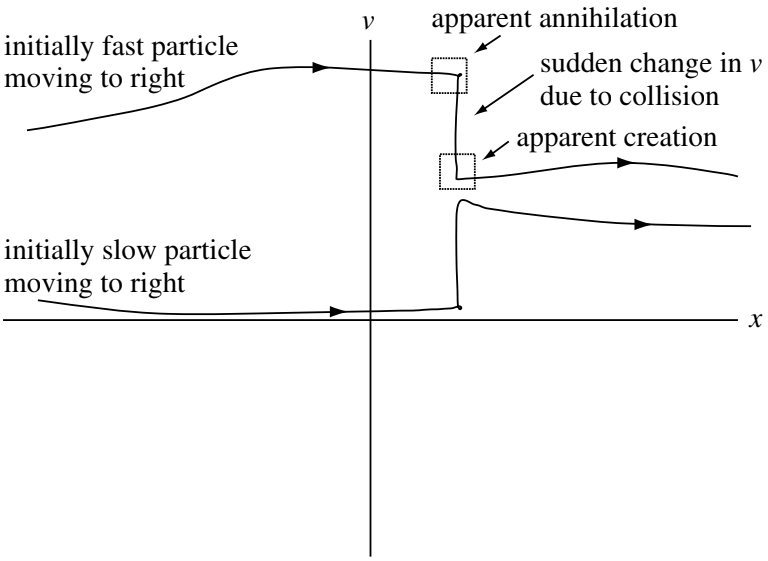
The details of these individual jumps in phase-space are complicated and yet of little interest since all we really want to know is the cumulative effect of many collisions. It is therefore both efficient and sufficient to follow the trajectories on the slow time scale while accounting for the apparent “creation” or “annihilation” of particles by inserting a collision operator on the right-hand side of the Vlasov equation. In the example shown here it is seen that when a particle is apparently “created” in one box, another particle must be simultaneously “annihilated” in another box at the same \(x\) coordinate but a different \(v\) coordinate (of course, what is actually happening is that a single particle is suddenly moving from one box to the other). This coupling of the annihilation and creation rates in different boxes constrains the form of the collision operator. We will not attempt to derive collision operators in this chapter but will simply discuss the constraints on these operators. From a more formal point of view, collisions are characterized by constrained sources and sinks for particles in phase-space and inclusion of collisions in the Vlasov equation causes the Vlasov equation to assume the form \[ \frac{\partial f_s}{\partial t} + \frac{\partial}{\partial\mathbf{x}}\cdot(\mathbf{v}f_s) + \frac{\partial}{\partial\mathbf{v}}\cdot(\mathbf{a}f_s) = \sum_\alpha C_{s\alpha}(f_s) \tag{12.13}\] where \(C_{s\alpha}(f_s)\) is the rate of change of \(f_s\) due to collisions of species \(s\) with species \(\alpha\)1. This is called the Boltzmann equation.
The constraints that must be satisfied by the collision operator \(C_{s\alpha}(f_s)\) are as follows:
Conservation of particles - Collisions cannot change the total number of particles at a particular location so \[ \int \mathrm{d}\mathbf{v} C_{s\alpha}(f_s) = 0 \tag{12.14}\]
Conservation of momentum - Collisions between particles of the same species cannot change the total momentum of that species so \[ \int \mathrm{d}\mathbf{v} m_s\mathbf{v}C_{ss}(f_s) = 0 \tag{12.15}\] while collisions between different species must conserve the total momentum of both species together so \[ \int \mathrm{d}\mathbf{v} m_i\mathbf{v}C_{ie}(f_i) + \int \mathrm{d}\mathbf{v} m_e\mathbf{v}C_{ei}(f_e) = 0 \tag{12.16}\]
Conservation of energy - Collisions between particles of the same species cannot change the total energy of that species so \[ \int \mathrm{d}\mathbf{v} m_s\mathbf{v}^2C_{ss}(f_s) = 0 \tag{12.17}\] while collisions between different species must conserve the total energy of both species together so \[ \int \mathrm{d}\mathbf{v} m_i\mathbf{v}^2C_{ie}(f_i) + \int \mathrm{d}\mathbf{v} m_e\mathbf{v}^2C_{ei}(f_e) = 0 \tag{12.18}\]
In a sufficiently hot plasma, collisions can be neglected. If, furthermore, the force \(\mathbf{F}\) is entirely electromagnetic, Equation 12.13 takes the special form of Equation 12.12. Because of its comparative simplicity, this is the equation most commonly studied in kinetic theory. When there are collisions with neutral atoms, the collision term in Equation 12.13 can be approximated by \[ \Big( \frac{\partial f}{\partial t} \Big)_c = \frac{f_n - f}{\tau} \] where \(f_n\) is the distribution function of the neutral atoms, and \(\tau\) is a constant collision time. This is called the Krook collision term. It is the kinetic generalization of the collision term in Eq. (5.5) in (Chen 2016). When there are Coulomb collisions, Equation 12.13 can be approximated by \[ \frac{\mathrm{d}f}{\mathrm{d}t} = -\frac{\partial}{\partial\mathbf{v}}\cdot(f\left<\Delta\mathbf{v}\right>)\frac{1}{2}\frac{\partial^2}{\partial\mathbf{v}\partial\mathbf{v}}:(f\left<\Delta\mathbf{v}\Delta\mathbf{v}\right>) \tag{12.19}\]
This is called the Fokker-Planck equation; it takes into account binary Coulomb collisions only. Here, \(\Delta\mathbf{v}\) is the change of velocity in a collision, and Equation 12.19 is a shorthand way of writing a rather complicated expression. The colon operator \(\mathbf{a}\mathbf{b}:\mathbf{c}\mathbf{d} = a_ib_jc_id_j\).
The fact that \(\mathrm{d}f/\mathrm{d}t\) is constant in the absence of collisions means that particles follow the contours of constant \(f\) as they move around in phase space. As an example of how these contours can be used, consider the beam-plasma instability of Section ???. In the unperturbed plasma, the electrons all have velocity \(v_0\), and the contour of constant \(f\) is a straight line. The function \(f(x, v_x)\) is a wall rising out of the plane of the paper at \(v_x=v_0\). The electrons move along the trajectory shown. When a wave develops, the electric field \(\mathbf{E}_1\) causes electrons to suffer changes in \(v_x\) as they stream along. The trajectory then develops a sinusoidal ripple (Figure 12.6 B). This ripple travels at the phase velocity, not the particle velocity. Particles stay on the curve as they move relative to the wave. If \(\mathbf{E}_1\) becomes very large as the wave grows, and if there are a few collisions, some electrons will be trapped in the electrostatic potential of the wave. In coordinate space, the wave potential appears as in Figure 12.7. In phase space, \(f(x, v_x)\) will have peaks wherever there is a potential trough (Figure 12.8). Since the contours of \(f\) are also electron trajectories, one sees that some electrons move in closed orbits in phase space; these are just the trapped electrons.


Electron trapping is a nonlinear phenomenon which cannot be treated by straightforward solution of the Vlasov equation. However, electron trajectories can be followed on a computer, and the results are often presented in the form of a plot like Figure 12.8.
ADD A TWO STREAM INSTABILITY PHASE ANIMATION!
12.4 Derivation of the Fluid Equations
Instead of just taking moments of the distribution function \(f\) itself, moments will now be taken of the entire Vlasov equation to obtain a set of partial differential equations relating the mean quantities \(n(\mathbf{x}),\mathbf{u}(\mathbf{x})\), etc. We begin by integrating the Vlasov equation, Equation 12.12, over velocity for each species. This first and simplest step in the procedure is called taking the “zeroth” moment, since the operation of multiplying by unity can be considered as multiplying the entire Vlasov equation by \(\mathbf{v}\) raised to the power zero. Multiplying the Vlasov equation by unity and then integrating over velocity gives \[ \int\left[ \frac{\partial f_s}{\partial t} + \frac{\partial}{\partial\mathbf{x}}\cdot(\mathbf{v}f_s) + \frac{\partial}{\partial\mathbf{v}}\cdot(\mathbf{a}f_s) \right]\mathrm{d}\mathbf{v} = \sum_\alpha \int C_{s\alpha}(f_s)\mathrm{d}\mathbf{v} \]
The velocity integral commutes with both the time and space derivatives on the left-hand side because \(\mathbf{x}, \mathbf{v}\) and \(t\) are independent variables, while the third term on the left-hand side is the volume integral of a divergence in velocity space. Gauss’ theorem (i.e., \(\int_V\mathrm{d}\mathbf{x}\nabla\cdot\mathbf{Q}=\int_A\mathrm{d}\mathbf{s}\cdot\mathbf{Q}\)) gives \(f_s\) evaluated on a surface at \(v=\infty\). However, because \(f_s\rightarrow 0\) as \(v\rightarrow\infty\), this surface integral in velocity space vanishes. Inserting Equation 12.1, Equation 12.4, and Equation 12.14 into the above, we have the species continuity equation \[ \frac{\partial n_s}{\partial t} + \nabla\cdot(n_s\mathbf{u}_s)=0 \tag{12.20}\]
Now let us multiply Equation 12.12 by \(\mathbf{v}\) and integrate over velocity to take the “first moment”, \[ \int \mathbf{v}\left[ \frac{\partial f_s}{\partial t} + \frac{\partial}{\partial\mathbf{x}}\cdot(\mathbf{v}f_s) + \frac{\partial}{\partial\mathbf{v}}\cdot(\mathbf{a}f_s) \right]\mathrm{d}\mathbf{v} = \sum_\alpha \int \mathbf{v}C_{s\alpha}(f_s)\mathrm{d}\mathbf{v} \]
This may be rearranged in a more tractable form by:
- pulling both the time and space derivatives out of the velocity integral,
- writing \(\mathbf{v} = \mathbf{v}^\prime(\mathbf{x},t) + \mathbf{u}(\mathbf{x},t)\), where \(\mathbf{v}^\prime(\mathbf{x},t)\) is the random part of a given velocity, i.e., that part of the velocity that differes from the mean (note that \(\mathbf{v}\) is independent of both \(\mathbf{x}\) and \(t\) but \(\mathbf{v}^\prime\) is not; also \(\mathrm{d}\mathbf{v}=\mathrm{d}\mathbf{v}^\prime\) since \(\mathbf{u}\) is independent of \(\mathbf{v}\)),
- integrating by parts in 3-D velocity space on the acceleration term and using \[ \partial_i\mathbf{v}_j = \delta_{ij} \]
After performing these manipulations, the first moment of the Vlasov equation becomes \[ \begin{aligned} \frac{\partial(n_s\mathbf{u}_s)}{\partial t} + \frac{\partial}{\partial\mathbf{x}}\cdot\int\left( \mathbf{v}^\prime\mathbf{v}^\prime + \mathbf{v}^\prime\mathbf{u}_s + \mathbf{u}_s\mathbf{v}^\prime +\mathbf{u}_s\mathbf{u}_s \right)f_s \mathrm{d}\mathbf{v}^\prime \\ - \frac{q_s}{m_s}\int \left( \mathbf{E}+\mathbf{v}\times\mathbf{B} \right)f_s\mathrm{d}\mathbf{v}^\prime = -\frac{1}{m_s}\mathbf{R}_{s\alpha} \end{aligned} \tag{12.21}\] where \(\mathbf{R}_{s\alpha}\) is the net frictional drag force due to collisions of species \(s\) with species \(\alpha\). Note that \(\mathbf{R}_{ss} = 0\), since a species cannot exert a net drag force on itself. The frictional terms have the form \[ \begin{aligned} \mathbf{R}_{ei} &= \nu_{ei}m_e n_e (\mathbf{u}_e - \mathbf{u}_i) \\ \mathbf{R}_{ie} &= \nu_{ie}m_i n_i (\mathbf{u}_i - \mathbf{u}_e) \end{aligned} \] so that in the ion frame the drag on electrons is simply the total electron momentum \(m_e n_e\mathbf{u}_e\) measured in this frame multiplied by the rate \(\nu_{ei}\) at which this momentum is destroyed by collisions with ions. This form for frictional drag force has the following properties: (i) \(\mathbf{R}_{ei} + \mathbf{R}_{ie} = 0\), showing that the plasma cannot exert a frictional drag force on itself, (ii) friction causes the faster species to be slowed down by the slower species, and (iii) there is no friction between species if both have the same mean velocity.
Equation 12.21 can be further simplified by factoring \(\mathbf{u}\) out of the velocity integrals and recalling that by definition \(\int \mathbf{v}^\prime f_s \mathrm{d}\mathbf{v}^\prime=0\). Thus Equation 12.21 reduces to \[ m_s\left[ \frac{\partial(n_s\mathbf{u}_s)}{\partial t} + \frac{\partial}{\partial\mathbf{x}}\cdot(n_s\mathbf{u}_s\mathbf{u}_s) \right] = n_s q_s (\mathbf{E} + \mathbf{u}_s\times\mathbf{B}) - \frac{\partial}{\partial\mathbf{x}}\cdot\overleftrightarrow{P}_s - \mathbf{R}_{s\alpha} \] where the pressure tensor is defined by \[ \overleftrightarrow{P}_s \equiv m_s\int \mathbf{v}^\prime \mathbf{v}^\prime f_s \mathrm{d}\mathbf{v}^\prime \tag{12.22}\]
If \(f_s\) is an isotropic function of \(\mathbf{v}^\prime\), then the off-diagonal terms in \(\overleftrightarrow{P}_s\) vanish and the three diagonal terms are identical. In this case, it is useful to define the diagonal terms to be the scalar pressure \(p_s\), i.e., \[ \begin{aligned} p_s &= m_s \int v_x^\prime v_x^\prime f_s \mathrm{d}\mathbf{v}^\prime = m_s \int v_y^\prime v_y^\prime f_s \mathrm{d}\mathbf{v}^\prime = m_s \int v_z^\prime v_z^\prime f_s \mathrm{d}\mathbf{v}^\prime \\ &= \frac{m_s}{3} \int \mathbf{v}^\prime\cdot \mathbf{v}^\prime f_s \mathrm{d}\mathbf{v}^\prime \end{aligned} \tag{12.23}\]
Equation 12.23 defines pressure for a three-dimensional isotropic system. However, we will often deal with systems of reduced dimensionality, i.e., systems with just one or two dimensions. Equation 12.23 can therefore be generalized to these other cases by introducing the general N-dimensional definition for scalar pressure \[ p_s = \frac{m_s}{N}\int \mathbf{v}^\prime\cdot \mathbf{v}^\prime f_s \mathrm{d}^N\mathbf{v}^\prime \tag{12.24}\] where \(\mathbf{v}^\prime\) is the N-dimensional random velocity.
The scalar pressure has a simple relation to the generalized Maxwellian as seen by recasting Equation 12.24 as \[ \begin{aligned} p_s &= \frac{m_s}{N}\int \mathbf{v}^\prime\cdot \mathbf{v}^\prime f_s \mathrm{d}^N\mathbf{v}^\prime \\ &= \frac{n_s m_s}{N}\left( \frac{m_s}{2\pi k_B T_s} \right)^{N/2} \int {\mathbf{v}^\prime}^2 \exp \left( -\frac{m_s {\mathbf{v}^\prime}^2}{2k_B T_s} \right) \mathrm{d}^N\mathbf{v}^\prime \\ &= -\frac{n_s m_s}{N}\left( \frac{\alpha}{\pi} \right)^{N/2} \frac{\mathrm{d}}{\mathrm{d}\alpha}\int e^{-\alpha {v^\prime}^2}\mathrm{d}^N\mathbf{v}^\prime,\, \alpha \equiv m_s/2k_B T_s \\ &= -\frac{n_s m_s}{N}\left( \frac{\alpha}{\pi} \right)^{N/2} \frac{\mathrm{d}}{\mathrm{d}\alpha}\left( \frac{\alpha}{\pi} \right)^{-N/2} \\ &= n_s k_B T_s \end{aligned} \] which is just the ideal gas law. Thus, the definitions that have been proposed for pressure and temperature are consistent with everyday notions for these quantities.
It is important to emphasize that assuming isotropy is done largely for mathematical convenience and that in real systems the distribution function is often quite anisotropic. Collisions, being randomizing, drive the distribution function towards isotropy, while competing processes simultaneously drive it towards anisotropy. Thus, each situation must be considered individually in order to determine whether there is sufficient collisionality to make \(f\) isotropic. Because fully ionized hot plasmas often have insufficient collisions to make \(f\) isotropic, the often-used assumption of isotropy is an oversimplification, which may or may not be acceptable depending on the phenomenon under consideration.
On expanding the derivatives on the left-hand side of Equation 12.21, it is seen that two of the terms combine to give \(\mathbf{u}\) times Equation 12.20. After removing this embedded continuity equation, E@eq-vlasov-1st-moment reduces to \[ n_s m_s\frac{\mathrm{d}\mathbf{u}_s}{\mathrm{d}t} = n_s q_s(\mathbf{E} + \mathbf{u}_s\times\mathbf{B}) - \nabla p_s - \mathbf{R}_{s\alpha} \] where the operator \(\mathrm{d}/\mathrm{d}t\) is the convective derivative (Equation 3.2).
At this point in the procedure it becomes evident that a certain pattern recurs for each successive moment of the Vlasov equation. When we took the zeroth moment, an equation for the density \(\int f\mathrm{d}\mathbf{v}\) resulted, but this also introduced a term involving the next higher moment, namely the mean velocity \(\sim\int\mathbf{v}f\mathrm{d}\mathbf{v}\). Then, when we took the first moment to get an equation for the velocity, an equation was obtained containing a term involving the next higher moment, namely the pressure \(\sim\int \mathbf{v}\mathbf{v}f\mathrm{d}\mathbf{v}\). Thus, each time we take a moment of the Vlasov equation, an equation for the moment we want is obtained, but because of the \(\mathbf{v}\cdot\nabla f\) term in the Vlasov equation, a next higher moment also appears. Thus, moment-taking never leads to a closed system of equations; there will always be a “loose end”, a highest moment for which there is no determining equation. Some sort of ad hoc closure procedure must always be invoked to terminate this chain (as seen below, typical closures involve invoking adiabatic or isothermal assumptions). Another feature of taking moments is that each higher moment embeds terms that contain complete lower moment equations multiplied by some factor. Algebraic manipulation can identify these lower moment equations and eliminate them to give a simplified higher moment equation.
Let us now take the second moment of the Vlasov equation. Unlike the zeroth and first moments, the dimensionality of the system now enters explicitly so the more general pressure definition given by Equation 12.24 will be used. Multiplying the Vlasov equation by \(m_s v^2/2\) and integrating over velocity gives \[ \begin{Bmatrix} \frac{\partial}{\partial t}\int \frac{m_s v^2}{2}f_s\mathrm{d}^N\mathbf{v} \\ +\frac{\partial}{\partial\mathbf{x}}\cdot\int\frac{m_s v^2}{2}\mathbf{v}f_s\mathrm{d}^N\mathbf{v} \\ +q_s\int\frac{v^2}{2}\frac{\partial}{\partial\mathbf{v}}\cdot(\mathbf{E}+\mathbf{v}\times\mathbf{B})f_s\mathrm{d}^N\mathbf{v} \end{Bmatrix} = \sum_\alpha \int m_s \frac{v^2}{2}C_{s\alpha}f_s\mathrm{d}^N \mathbf{v} \tag{12.25}\]
We consider each term of this equation separately as follows:
The time derivative term becomes \[ \frac{\partial}{\partial t}\int \frac{m_s v^2}{2}f_s\mathrm{d}^N\mathbf{v} = \frac{\partial}{\partial t}\int \frac{m_s(\mathbf{v}^\prime + \mathbf{u}_s)^2}{2} f_s\mathrm{d}^N\mathbf{v}^\prime = \frac{\partial}{\partial t}\left( \frac{Np_s}{2} + \frac{m_sn_su_s^2}{2} \right) \]
Again using \(\mathbf{v}=\mathbf{v}^\prime + \mathbf{u}_s\), the space derivative term becomes \[ \frac{\partial}{\partial\mathbf{x}}\cdot\int\frac{m_s v^2}{2}\mathbf{v}f_s\mathrm{d}^N\mathbf{v} = \nabla\cdot\left( \mathbf{Q}_s + \frac{2+N}{2}p_s\mathbf{u}_s + \frac{m_sn_su_s^2}{2}\mathbf{u}_s \right) \] where \[ \mathbf{Q}_s = \int\frac{m_s{v^\prime}^2}{2}\mathbf{v}^\prime f_s\mathrm{d}^N\mathbf{v} \] is called the heat flux.
On integrating by parts, the acceleration term becomes \[ q_s\int\frac{v^2}{2}\frac{\partial}{\partial\mathbf{v}}\cdot(\mathbf{E}+\mathbf{v}\times\mathbf{B})f_s\mathrm{d}^N\mathbf{v} = -q_s\int\mathbf{v}\cdot\mathbf{E} f_s\mathrm{d}\mathbf{v} = -q_s n_s\mathbf{u}_s\cdot\mathbf{E} \]
The collision term becomes (using Equation 12.17) \[ \sum_\alpha \int m_s \frac{v^2}{2}C_{s\alpha}f_s\mathrm{d}^N \mathbf{v} = \int_{s\neq \alpha}m_s\frac{v^2}{2}C_{s\alpha} f_s\mathrm{d}\mathbf{v} = -\left( \frac{\partial W}{\partial t} \right)_\mathrm{Es\alpha} \] where \((\partial W/\partial t)_\mathrm{Es\alpha}\) is the rate at which species \(s\) collisionally transfers energy to species \(\alpha\).
Combining the above four relations, Equation 12.25 becomes \[ \begin{aligned} \frac{\partial}{\partial t}\left( \frac{Np_s}{2} + \frac{m_sn_su_s^2}{2} \right) + \nabla\cdot\left( \mathbf{Q}_s +\frac{2+N}{2}p_s\mathbf{u}_s + \frac{m_sn_su_s^2}{2}\mathbf{u}_s \right) - q_s n_s \mathbf{u}_s\cdot\mathbf{E} \\ = -\left( \frac{\partial W}{\partial t} \right)_\mathrm{E\sigma s} \end{aligned} \tag{12.26}\]
This equation can be simplified by invoking two mathmatical identities, the first being \[ \frac{\partial}{\partial t}\left( \frac{m_s n_s u_s^2}{2} \right) + \nabla\cdot\left( \frac{m_sn_su_s^2}{2}\mathbf{u}_s \right) = n_s\left( \frac{\partial}{\partial t} + \mathbf{u}_s\cdot\nabla \right)\frac{m_su_s^2}{2} = n_s\frac{\mathrm{d}}{\mathrm{d}t}\left( \frac{m_su_s^2}{2} \right) \]
The second identity is obtained by dotting the equation of motion with \(\mathbf{u}_s\): \[ \begin{aligned} n_s m_s\left[ \frac{\partial}{\partial t}\left( \frac{u_s^2}{2}\right) + \mathbf{u}_s\cdot\left( \nabla\left( \frac{u_s^2}{2} \right) - \mathbf{u}_s\times\nabla\times\mathbf{u}_s \right) \right] \\ = n_s q_s \mathbf{u}_s\cdot\mathbf{E} - \mathbf{u}_s\cdot\nabla p_s - \mathbf{R}_{s\alpha}\cdot\mathbf{u}_s \end{aligned} \] or \[ n_s\frac{\mathrm{d}}{\mathrm{d}t}\left( \frac{m_su_s^2}{2} \right) = n_sq_s\mathbf{u}_s\cdot\mathbf{E} - \mathbf{u}_s\cdot\nabla p_s - \mathbf{R}_{s\alpha}\cdot\mathbf{u}_s \]
Inserting these two into Equation 12.26 gives the energy evolution equation \[ \frac{N}{2}\frac{\mathrm{d}p_s}{\mathrm{d}t} + \frac{2+N}{2}p_s\nabla\cdot\mathbf{u}_s = -\nabla\cdot\mathbf{Q}_s + \mathbf{R}_{s\alpha}\cdot\mathbf{u}_s - \left(\frac{\partial W}{\partial t}\right)_\mathrm{Es\alpha} \tag{12.27}\]
The first term on the right-hand side represents the heat flux, the second term gives the frictional heating of species \(s\) due to frictional drag on species \(\alpha\), while the last term on the right-hand side gives the rate at which species \(s\) collisionally transfers energy to other species. Although Equation 12.27 is complicated, two important limiting situations become evident if we let \(t_\mathrm{char}\) be the characteristic time scale for a given phenomenon and \(l_\mathrm{char}\) be its characteristic length scale. A characteristic velocity \(V_\mathrm{ph}\sim l_\mathrm{char}/t_\mathrm{char}\) may then be defined for the phenomenon and so, replacing temporal derivatives by \(t_\mathrm{char}^{-1}\) and spatial derivatives by \(l_\mathrm{char}^{-1}\) in Equation 12.27, it is seen that the two limiting situations are:
Isothermal limit - The heat flux term dominates all other terms, in which case the temperature becomes spatially uniform. This occurs if (i) \(v_{Ts}\gg V_\mathrm{ph}\) since the ratio of the left-hand side terms to the heat flux term is \(\sim V_\mathrm{ph}/v_{Ts}\) and (ii) the collisional terms are small enough to be ignored.
Adiabatic limit - The heat flux terms and the collisional terms are small enough to be ignored compared to the left-hand side terms; this occurs when \(V_\mathrm{ph} \gg v_{Ts}\). Adiabatic is a Greek word meaning “impassable”, and is used here to denote that no heat is flowing, i.e., the volume under consideration is thermally isolated from the outside world.
Both of these limits make it possible to avoid solving for \(\mathbf{Q}_s\), which involves the third moment, and so both the adiabatic and isothermal limit provide a closure to the moment equations.
The energy equation may be greatly simplified in the adiabatic limit by re-arranging the continuity equation to give \[ \nabla\cdot\mathbf{u}_s = -\frac{1}{n_s}\frac{\mathrm{d}n_s}{\mathrm{d}t} \] and then substituting this expression into the left-hand side of Equation 12.27 to obtain \[ \frac{1}{p_s}\frac{\mathrm{d}p_s}{\mathrm{d}t} = \frac{\gamma}{n_s}\frac{\mathrm{d}n_s}{\mathrm{d}t} \tag{12.28}\] where \[ \gamma = \frac{N+2}{N} \]
Equation 12.28 implies \[ \frac{\mathrm{d}}{\mathrm{d}t}\left( \frac{p_s}{n_s^\gamma} \right) = 0 \] so \(p_s/n_s^\gamma\) is a constant in the frame of the moving plasma. This constitutes a derivation of adiabaticity based on geometry and statistical mechanics rather than on thermodynamic arguments.
The energy equation derivation can also be found in An introductory guide to fluid models with anisotropic temperatures.
As a short summary, the fluid equations we have been using are simply moments of the Boltzmann equation. One interesting observation from Equation 12.12 is that in order to recover the hydrodynamic equations, the acceleration term \(\mathbf{a}\cdot\partial_\mathbf{v}f\) is not required: the pressure gradient that drives the flow arises from the thermal motion embedded in the advection term \(\mathbf{v}\cdot\partial_\mathbf{x}f\).
We must be careful not to become overconfident regarding the descriptive power of the fluid point of view because weaknesses exist in this point of view. For example, as discussed above neither the adiabatic nor the isothermal approximation is appropriate when \(V_\mathrm{ph}\sim v_{Ts}\). The fluid description breaks down in this situation and the Vlasov description must be used in this situation. Furthermore, the distribution function is Maxwellian only if there are sufficient collisions or some other randomizing process. Because of the weak collisionality of a plasma, this is very often not the case. In particular, since the collision frequency scales as \(v^{-3}\) (Equation 9.20), fast particles take much longer to become Maxwellian than slow particles. It is not at all unusual for a real plasma to be in a state where the low-velocity particles have reached a Maxwellian distribution whereas the fast particles form a non-Maxwellian tail.
12.5 Plasma Oscillations and Landau Damping
As an elementary illustration of the use of the Vlasov equation, we shall derive the dispersion relation for electron plasma oscillations, which is originally treated from the fluid point of view. This derivation will require a knowledge of contour integration.
In zeroth order, we assume a uniform plasma with a distribution \(f_0(\mathbf{v})\), and we let \(\mathbf{B}_0 = \mathbf{E}_0 = 0\). In first order, we denote the perturbation in \(f(\mathbf{r},\mathbf{v},t)\) by \(f_1(\mathbf{r},\mathbf{v},t)\):
\[ f(\mathbf{r},\mathbf{v},t) = f_0(\mathbf{v}) + f_1(\mathbf{r},\mathbf{v},t) \]
Since \(\mathbf{v}\) is now an independent variable and is not to be linearized, the first-order Vlasov equation for electron is
\[ \frac{\partial f_1}{\partial t} + \mathbf{v}\cdot\nabla f_1 - \frac{e}{m}\mathbf{E}_1\cdot\frac{\partial f_0}{\partial \mathbf{v}} = 0 \tag{12.29}\]
As before, we assume the ions are massive and fixed and that the waves are plane waves in the x direction \(f_1 \propto e^{i(kx - \omega t)}\). Then the linearized Vlasov equation becomes
\[ \begin{aligned} -i\omega f_1 + ikv_x f_1 x &= \frac{e}{m}E_x\frac{\partial f_0}{\partial v_x} \\ f_1 &= \frac{ieE_x}{m}\frac{\partial f_0/\partial v_x}{\omega - kv_x} \end{aligned} \]
Poisson’s equation gives \[ \epsilon_0\nabla\cdot\mathbf{E}_1 = ik\epsilon_0 E_x = -en_1 = -e\int f_1 d^3v \]
Substituting for \(f_1\) and dividing by \(ik\epsilon_0 E_x\), we have \[ 1 = -\frac{e^2}{km\epsilon_0}\int \frac{\partial f_0/\partial v_x}{\omega - k v_x}d^3v \]
A factor \(n_0\) can be factored out if we replace \(f_0\) by a normalized function \(\hat{f}_0\): \[ 1 = -\frac{\omega_p^2}{k}\int_{-\infty}^{\infty}dv_z\int_{-\infty}^{\infty}dv_y\int_{-\infty}^{\infty}\frac{\partial \hat{f}_0(v_x, v_y, v_z)/\partial v_x}{\omega- k v_x}dv_x \]
If \(f_0\) is a Maxwellian or some other factorable distribution, the integration over \(v_y\) and \(v_z\) can be carried out easily. What remains is the one-dimensional distribution \(\hat{f}_0(v_x)\). For instance, a one-dimensional Maxwellian distribution is \[ \hat{f}_m(v_x) = \sqrt{\frac{m}{2\pi k_B T}} \exp\left(\frac{-mv_x^2}{2 k_B T}\right) \]
Since we are dealing with a one-dimensional problem we may drop the subscript x, begin careful not to confuse \(v\) (which is really \(v_x\)) with the total velocity \(v\) used earlier: \[ 1 = \frac{\omega_p^2}{k^2}\int_{-\infty}^{\infty}\frac{\partial \hat{f}_0/\partial v}{v - \omega/k}\mathrm{d}v \tag{12.30}\]
Here, \(\hat{f}_0\) is understood to be a one-dimensional distribution function, the integrations over \(v_y\) and \(v_z\) having been made. This equation holds for any equilibrium distribution \(\hat{f}_0(v)\).
The integral in this equation is not straightforward to evaluate because of the singularity at \(v=\omega/k\). One might think that the singularity would be of no concern, because in practice \(\omega\) is almost always never real; waves are usually slightly damped by collisions or are amplified by some instability mechanisms. Since the velocity \(v\) is a real quantity, the denominator never vanishes. Landau was the first to treat this equation properly. He found that even though the singularity lies off the path of integration, its presence introduces an important modification to the plasma wave dispersion relation — an effect not predicted by the fluid theory.
Consider an initial value problem in which the plasma is given a sinusoidal perturbation, and therefore \(k\) is real. If the perturbation grows or decays, \(\omega\) will be complex. This integral must be treated as a contour integral in the complex \(v\) plane. Possible contours are shown for (a) an unstable wave, with \(\Im(\omega) > 0\), and (b) a dampled wave, with \(\Im(\omega) < 0\). Normally, one would evaluate the line integral along the real \(v\) axis by the residue theorem: \[ \int_{C_1} G \mathrm{d}v + \int_{C_2} G \mathrm{d}v = 2\pi i R(\omega/k) \] where \(G\) is the integrand, \(C_1\) is the path along the real axis, \(C_2\) is the semicircle at infinity, and \(R(\omega/k)\) is the residue at \(\omega/k\). This works if the integral over \(C_2\) vanishes. Unfortunately, this does not happen for a Maxwellian distribution, which contains the factor \[ \exp(-v^2/v_{th}^2) \]
This factor becomes large for \(v\rightarrow \pm i \infty\), and the contribution from \(C_2\) cannot be neglected. Landau showed that when the problem is properly treated as an initial value problem the correct contour to use is the curve \(C_1\) passing below the singularity. This integral must in general be evaluated numerically.
Although an exact analysis of this problem is complicated, we can obtain an approximate dispersion relation for the case of large phase velocity and weak damping. In this case, the pole at \(\omega/k\) lies near the real \(v\) axis. The contour prescribed by Landau is then a straight line along the \(\Re(v)\) axis with a small semicircle around the pole. In going around the pole, one obtains \(2\pi i\) time half the residue there. Then Equation 12.30 becomes \[ 1 = \frac{\omega_p^2}{k^2} \left[ P\int_{-\infty}^{\infty}\frac{\partial\hat{f}_0/\partial v}{v - (\omega/k)}\mathrm{d}v + i\pi \frac{\partial\hat{f}_0}{\partial v}\biggr\rvert_{v=\omega/k} \right] \tag{12.31}\] where \(P\) stands for the Cauchy principal value. To evaluate this, we integrate along the real \(v\) axis but stop just before encountering the pole. If the phase velocity \(v_\phi = \omega/k\) is sufficiently large, as we assume, there will not be much contribution from the neglected part of the contour, since both \(\hat{f}_0\) and \(\partial\hat{f}_0/\partial v\) are very small there. The integral above can be evaluated by integration by parts: \[ \int_{-\infty}^{\infty}\frac{\partial\hat{f}_0}{\partial v}\frac{\mathrm{d}v}{v - v_\phi} = \left[ \frac{\hat{f}_0}{v-v_\phi} \right]_{-\infty}^{\infty} - \int_{-\infty}^{\infty}\frac{-\hat{f}_0 \mathrm{d}v}{(v-v_\phi)^2} = \int_{-\infty}^{\infty}\frac{\hat{f}_0 \mathrm{d}v}{(v-v_\phi)^2} \]
Since this is just an average of \((v-v_\phi)^{-2}\) over the distribution, the real part of the dispersion relation can be written \[ 1 = \frac{\omega_p^2}{k^2} \overline{(v-v_\phi)^{-2}} \]
Since \(v_\phi \gg v\) has been assumed, we can expand \((v-v_\phi)^{-2}\): \[ (v-v_\phi)^{-2} = v_\phi^{-2}\Big( 1 - \frac{v}{v_\phi} \Big)^{-2} = v_\phi^{-2}\Big( 1 + \frac{2v}{v_\phi} + \frac{3v^2}{v_\phi^2} + \frac{4v^3}{v_\phi^3} + ... \Big) \]
The odd terms vanish upon taking the average, and we have \[ \overline{(v-v_\phi)^{-2}} \approx v_\phi^{-2} \Big( 1 + \frac{3\overline{v^2}}{v_\phi^2} \Big) \]
We now let \(\hat{f}_0\) be Maxwellian and evaluate \(\overline{v^2}\). Remembering that \(v\) here is an abbreviation for \(v_x\), we can write \[ \frac{1}{2}m\overline{v_x^2} = \frac{1}{2}k_B T_e \] there being only one degree of freedom. The dispersion relation then becomes \[ \begin{aligned} 1 &= \frac{\omega_p^2}{k^2}\frac{k^2}{\omega^2}\Big( 1+ 3\frac{k^2}{\omega^2}\frac{k_B T_e}{m} \Big) \\ \omega^2 &= \omega_p^2 + \frac{\omega_p^2}{\omega^2}\frac{3k_B T_e}{m}k^2 \end{aligned} \]
If the thermal correction is small (i.e. the second term on the right-hand side is small, such that \(\omega \approx \omega_p\)), we may replace \(\omega^2\) by \(\omega_p^2\) in the second term. We then have \[ \omega^2 = \omega_p^2 + \frac{3k_B T_e}{m}k^2 \] which is the same as that been obtained from the fluid equations with \(\gamma=3\).
We now return to the imaginary term in the dispersion relation. In evaluating this small term, it will be sufficiently accurate to neglect the thermal correction to the real part of \(\omega\) and let \(\omega^2\approx \omega_p^2\). From the evaluation of the real part above we see that the principle value of the integral is approximately \(k^2/\omega^2\). The dispersion relation now becomes \[ 1 = \frac{\omega_p^2}{\omega^2} + i\pi\frac{\omega_p^2}{k^2}\frac{\partial\hat{f}_0}{\partial v}\biggr\rvert_{v=v_\phi} \]
\[ \omega^2 \Big( 1 - i\pi\frac{\omega_p^2}{k^2}\frac{\partial\hat{f}_0}{\partial v}\biggr\rvert_{v=v_\phi} \Big) = \omega_p^2 \]
Treating the imaginary term as small, we can bring it to the right-hand side and take the square root by Taylar series expansion. We then obtain \[ \omega = \omega_p\Big( 1 + i\frac{\pi}{2}\frac{\omega_p^2}{k^2}\frac{\partial\hat{f}_0}{\partial v}\biggr\rvert_{v=v_\phi} \Big) \tag{12.32}\]
If \(\hat{f}_0\) is a one-dimensional Maxwellian, we have \[ \frac{\partial\hat{f}_0}{\partial v} = (\pi v_{th}^2)^{-1/2} \left( \frac{-2v}{v_{th}^2} \right) \exp\left( \frac{-v^2}{v_{th}^2} \right) = -\frac{2v}{\sqrt{\pi}v_{th}}\exp\left( \frac{-v^2}{v_{th}^2} \right) \]
We may approximate \(v_\phi\) by \(\omega_p/k\) in the coefficient, but in the exponent we must keep the thermal correction in the real part of the dispersion relation. The damping is then given by \[ \begin{aligned} \Im(\omega) &= -\frac{\pi}{2}\frac{\omega_p^2}{k^2}\frac{2\omega_p}{k\sqrt{\pi}}\frac{1}{v_{th}^3}\exp\left( \frac{-\omega^2}{k^2 v_{th}^2} \right) \\ &= -\sqrt{\pi}\omega_p \left( \frac{\omega_p}{kv_{th}} \right)^3 \exp\left( \frac{-\omega_p^2}{k^2 v_{th}^2}\right)\exp\left( \frac{-3}{2} \right) \\ \Im\left(\frac{\omega}{\omega_p}\right) &= -0.22 \sqrt{\pi}\left( \frac{\omega_p}{kv_{th}} \right)^3 \exp\left( \frac{-1}{2k^2\lambda_D^2} \right) \end{aligned} \]
Since \(\Im(\omega)\) is negative, there is a collisionless damping of plasma waves; this is called Landau damping. As is evident from the expression, this damping is extremely small for small \(k\lambda_D\), but becomes important for \(k\lambda_D = \mathcal{O}(1)\). This effect is connected with \(f_1\), the distortion of the distribution function caused by the wave.
12.6 The Meaning of Landau Damping
The theoretical discovery of wave damping without energy dissipation by collisions is perhaps the most astounding result of plasma physics research. That this is a real effect has been demonstrated in the laboratory. Although a simple physical explanation for this damping is now available, it is a triumph of applied mathematics that this unexpected effect was first discovered purely mathematically in the course of a careful analysis of a contour integral. Landau damping is a characteristic of collisionless plasmas, but it may also have application in other fields. For instance, in the kinetic treatment of galaxy formation, stars can be considered as atoms of a plasma interacting via gravitational rather than electromagnetic forces. Instabilities of the gas of stars can cause spiral arms to form, but this process is limited by Landau damping.
To see what is responsible for Landau damping, we first notice that \(\Im(\omega)\) arises from the pole at \(v=v_\phi\). Consequently, the effect is connected with those particles in the distribution that have a velocity nearly equal to the phase velocity — the “resonant particles”. These particles travel along with the wave and do not see a rapidly fluctuating electric field: they can, therefore, exchange energy with the wave effectively. The easiest way to understand this exchange of energy is to picture a surfer trying to catch an ocean wave. (Warning: this picture is only for directing our thinking along the right lines; it does not correctly explain the damping.) If the surfboard is not moving, it merely bobs up and down as the wave goes by and does not gain any energy on the average. Similarly, a boat propelled much faster than the wave cannot exchange much energy with the wave. However, if the surfboard has almost the same velocity as the wave, it can be caught and pushed along by the wave; this is, after all, the main purpose of the exercise. In that case, the surfboard gains energy, and therefore the wave must lose energy and is damped. On the other hand, if the surfboard should be moving slightly faster than the wave, it would push on the wave as it moves uphill; then the wave could gain energy. In a plasma, there are electrons both faster and slower than the wave. A Maxwellian distribution, however, has more slow electrons than fast ones. Consequently, there are more particles taking energy from the wave than vice versa, and the wave is damped. As particles with \(v\approx v_\phi\) are trapped in the wave, \(f(v)\) is flattened near the phase velocity. This distortion is \(f_1(v)\) which we calculated. As seen in Fig (ADD IT!), the perturbed distribution function contains the same number of particles but has gained total energy (at the expense of the wave).
From this discussion, one can surmise that if \(f_0(v)\) contained more fast particles than slow particles, a wave can be excited. Indeed, from the expression of \(\omega\) above, it is apparent that \(\Im(\omega)\) is positive if \(\partial\hat{f}_0/\partial v\) is positive at \(v=v_\phi\). Such a distribution is shown in Fig.7-19 (ADD IT!). Waves with \(v_\phi\) in the region of positive slope will be unstable, gaining energy at the expense of the particles. This is just the finite-temperature analogy of the two stream instability. When there are two cold (\(k_B T=0\)) electron streams in motion, \(f_0(v)\) consists of two \(\delta\)-functions. This is clearly unstable because \(\partial f_0/\partial v\) is infinite; and indeed, we found the instability from fluid theory. When the streams have fnite temperature, kinetic theory tells us that the relative densities and temperatures of the two stream must be such as to have a region of positive \(\partial f_0(v)/\partial v\) between them; more precisely, the total distribution function must have a minimum for instability.
The physical picture of a surfer catching waves is very appealing, but it is not precise enough to give us a real understanding of Landau damping. There are actually two kinds of Landau damping. Both kinds are independent of dissipative collisional mechanisms. If a particle is caught in the potential well of a wave, the phenomenon is called “trapping”. As in the case of a surfer, particles can indeed gain or lose energy in trapping. However, trapping does not lie within the purview of the linear theory. That this is true can be seen from the equation of motion \[ m\ddot{x} = qE(x) \]
If one evaluates \(E(x)\) by inserting the exact value of \(x\), the equation would be nonlinear, since \(E(x)\) is somehting like \(\sin kx\). What is done in linear theory is to use for \(x\) the unperturbed orbit; i.e. \(x=x_0 + v_0 t\). Then this becomes linear. This approximation, however, is no longer valid when a particle is trapped. When it encounters a potential hill large enough to reflect it, its velocity and position are, of course, greatly affected by the wave and are not close to their unperturbed values. In fluid theory, the equation of motion is \[ m\left[ \frac{\partial\mathbf{v}}{\partial t}+(\mathbf{v}\cdot\nabla)\mathbf{v} \right] = q\mathbf{E}(x) \]
Here, \(\mathbf{E}(x)\) is to be evaluated in the laboratory frame, which is easy; but to make up for it, there is the \((\mathbf{v}\cdot\nabla)\mathbf{v}\) term. The neglect of \((\mathbf{v}_1\cdot\nabla)\mathbf{v}_1\) in linear theory amounts to the same thing as using unperturbed orbits. In kinetic theory, the nonlinear term that is neglected is, from the first-order Vlasov Equation 12.29, \[ \frac{q}{m}E_1\frac{\partial f_1}{\partial v} \]
When the particles are trapped, they reverse their direction of travel relative to the wave, so the distribution function \(f(v)\) is greatly disturbed near \(v=\omega/k\). This means that \(\partial f_1/\partial v\) is comparable to \(\partial f_0/\partial v\), and the term above is not negligible. Hence, trapping is not in the linear theory.
When a wave grows to a large amplitude, collisionless damping with trapping does occur. One then finds that the wave does not decay monotonically; rather, the amplitude fluctuates during the decay as the trapped particles bounce back and forth in the potential wells. This is nonlinear Landau damping. Since the result before was derived from a linear theory, it must arise from a different physical effect. The question is: can untrapped electrons moving close to the phase velocity of the wave exchange energy with the wave? Before giving the answer, let us examine the energy of such electrons.
12.6.1 The Kinetic Energy of a Beam of Electrons
We may divide the electron distribution \(f_0(v)\) into a large number of monoenergetic beams. Consider one of these beams: it has unperturbed velocity \(u\) and density \(n_u\). The velocity \(u\) may lie near \(v_\phi\), so that this beam may consist of resonant electrons. We now turn on a plasma oscillation \(E(x,t)\) and consider the kinetic energy of the beam as it moves through the crests and troughs of the wave. The wave is caused by a self-consistent motion of all the beams together. If \(n_u\) is small enough (the number of beams large enough), the beam being examined has a negligible effect on the wave and may be considered as moving in a given field \(E(x,t)\). Let \[ \begin{aligned} E &= E_0\sin(kx-\omega t) = -d\phi/\mathrm{d}t \\ \phi &= (E_0/k)\cos(kx-\omega t) \end{aligned} \]
The linearized fluid equation for the beam is \[ m\left(\frac{\partial v_1}{\partial t} + u\frac{\partial v_1}{\partial x} \right) = -eE_0\sin(kx-\omega t) \]
A possible solution is \[ v_1 = -\frac{eE_0}{m}\frac{\cos(kx-\omega t)}{\omega-ku} \]
This is the velocity modulation caused by the wave as the beam electrons move past. To conserve particle flux, there is a corresponding oscillation in density, given by the linearized continuity equation:
\[ \frac{\partial n_1}{\partial t} + u\frac{\partial n_1}{\partial x} = -n_u\frac{\partial v_1}{\partial x} \]
Since \(v_1\) is proportional to \(\cos(kx-\omega t)\), we can try \(n_1 = \bar{n}_1 \cos(kx-\omega t)\). Substitution of this into the above yields \[ n_1 = -n_u\frac{eE_0 k}{m}\frac{\cos(kx-\omega t)}{(\omega-ku)^2} \]
(\(n_1\) and \(v_1\) can be shown in a series of phase relation plots as in Fig.7-21)(ADD IT!) one wavelength of \(E\) and of the potential \(-e\phi\) seen by the beam electrons.
We may now compute the kinetic energy \(W_k\) of the beam: \[ \begin{aligned} W_k &= \frac{1}{2}m(n_u+n_1)(u+v_1)^2 \\ &= \frac{1}{2}m(n_u u^2 + n_uv_1^2 +2un_1v_1 + n_1u^2 + 2n_uuv_1 + n_1v_1^2) \end{aligned} \]
The last three terms contain odd powers of oscillating quantites, so they will vanish when we average over a wavelength. The change in \(W_k\) due to the wave is found by subtracting the first term, which is the original energy. The average energy change is then \[ \left<\Delta W_k \right> = \frac{1}{2}m\left<n_uv_1^2 + 2un_1v_1\right> \]
From the form of \(v_1\), we have \[ n_u\left< v_1^2 \right> = \frac{1}{2}n_u\frac{e^2E_0^2}{m^2(\omega-ku)^2} \] the factor \(\frac{1}{2}\) representing \(\left< \cos^2(kx-\omega t) \right>\). Similarly, from the form of \(n_1\), \[ 2u\left< n_1v_1 \right> = n_u\frac{e^2E_0^2 ku}{m^2(\omega - ku)^3} \]
Consequently, \[ \begin{aligned} \left<\Delta W_k \right> &= \frac{1}{4}mn_u \frac{e^2E_0^2}{m^2(\omega - ku)^2}\Big[ 1+\frac{2ku}{\omega-ku} \Big] \\ &= \frac{n_u}{4}\frac{e^2E_0^2}{m}\frac{\omega+ku}{m^2(\omega - ku)^3} \end{aligned} \]
This result shows that \(\left<\Delta W_k\right>\) depends on the frame of the observer and that it does not change secularly with time. Consider the picture of a frictionless block sliding over a washboard-like surface. (ADD FIGURE!) In the frame of the washboard, \(\left<\Delta W_k \right>\) is proportional to \(-(ku)^{-2}\), as seen by taking \(\omega = 0\). It is intuitively clear that (1) \(\left<\Delta W_k \right>\) is negative, since the block spends more time at the peaks than at the valleys, and (2) the block does not gain or lose energy on the average, once the oscillation is started (no time-dependence). Now if one goes into a frame in which the washboard is movign with a steady velocity \(\omega/k\) (a velocity unaffected by the motion of the block, since we have assumed that \(n_u\) is negligibly small compared with the density of the whole plasma), it is still true that the block does not gain or lose energy on the average, once the oscillation is started. But the above equation tells us that \(\left<\Delta W_k\right>\) depends on the velocity \(\omega/k\), and hence on the frame of the observer. In particular, it shows that a beam has less energy in the presence of the wave than in its absence if \(\omega - ku<0\) or \(u>u_\phi\), and it has more energy if \(\omega - ku>0\) or \(u<u_\phi\). The reason for this can be traced back to the phase relation between \(n_1\) and \(v_1\). As Fig.7-23 (ADD IT!) shows, \(W_k\) is a parabolic function of \(v\). As \(v\) oscillates between \(u-|v_1|\) and \(u+|v_1|\), \(W_k\) will attain an average value larger than the equilibrium value \(W_{k0}\), provided that the particle spends an equal amount of time in each half of the oscillation. This effect is the meaning of the first term \(\frac{1}{2}m\left< n_uv_1^2 \right>\), which is positive definite. The second term \(\frac{1}{2}m\left< 2un_1v_1 \right>\) is a correction due to the fact that the particle does not distribution its time equally. In Fig.7-21 (ADD IT!), one sees that both electrons a and b spend more time at the top the potential hill than at the bottom, but electron a reaches that point after a period of deceleration, so that \(v_1\) is negative there, while electron b reaches that point after a period of acceleration (to the right), so that \(v_1\) is positive there. This effect causes \(\left<W_k\right>\) to change sign at \(u=v_\phi\).
12.6.2 The Effect of Initial Conditions
The result we have just derived, however, still has nothing to do with linear Landau damping. Damping requires a continuous increase of \(W_k\) at the expense of wave energy, but we have found that \(\left<\Delta W_k\right>\) for untrapped particles is contant in time. If neither the untrapped particles nor the trapped particles are responsible for linear Landau damping, what is? The answer can be gleaned form the following observation: if \(\left<\Delta W_k\right>\) is positive, say, there must have been a time when it was increasing. Indeed, there are particles in the original distribution which have velocities so close to \(v_\phi\) that at time \(t\) they have not yet gone a half wavelength relative to the wave. For these particles, one cannot take the average \(\left<\Delta W_k\right>\). These particles can absorb energy from the wave and are properly called the “resonant” particles. As time goes on, the number of resonant electrons decreases, since an increasing number will have shifted more than \(\frac{1}{2}\lambda\) from their orginal positions. The damping rate, however, can stay constant, since the amplitude is now smaller, and it takes fewer electrons to maintain a constant damping rate.
The effect of the initial conditions is most easily seen form a phase-space diagram (Fig.7-24)(ADD IT with Luxor?).
12.7 A Physical Derivation of Landau Damping
We are now in a position to derive the Landau damping rate recourse to contour integration. Although Landau’s derivation of collisionless damping was short and neat, it was not clear that it concerned a physically observable phenomenon until J. M. Dawson gave the longer, intuitive derivation which is paraphrased in this section. As before, we divide the plasma up into beams of velocity \(u\) and density \(n_u\), and examine their motion in a wave
\[ E = E_1 \sin(kx-\omega t) \]
From the derivations in the previous section, the velocity of each beam is
\[ v_1 = -\frac{eE_1}{m}\frac{\cos(kx-\omega t)}{\omega-ku} \]
This solution satisfies the equation of motion, but it does not satisfy the initial condition \(v_1 = 0\) at \(t = 0\). It is clear that this initial condition must be imposed; otherwise, \(v_1\) would be very large in the vicinity of \(u=\omega/k\), and the plasma would be in a specially prepared state initially. We can fix up the solution to satisfy the initial condition by adding an arbitrary function of \(kx-kut\). The composite solution would still satisfy the equation of motion because the operator on the left-hand side, when applied to \(f(kx-kut)\), gives zero. Obviously, to get \(v_1 = 0\) at \(t=0\), the function \(f(kx-kut)\) must be taken to be \(-\cos(kx-kut)\). Thus we have, instead of the expression above,
\[ v_1 = \frac{-eE_1}{m}\frac{\cos(kx-\omega t) - \cos(kx-kut)}{\omega-ku} \]
Next, we must solve the equation of continuity for \(n_1\), again subject to the initial condition \(n_1=0\) at \(t=0\). Since we are now much cleverer than before, we may try a solution of the form
\[ n_1 = \bar{n}_1[\cos(kx-\omega t) - \cos(kx-kut)] \]
Inserting this into the equation of continuity and using the expression for \(v_1\) above, we find
\[ \bar{n}_1 \sin(kx-\omega t) = -n_u\frac{eE_1 k}{m}\frac{\sin(kx-\omega t) - \sin(kx-kut)}{(\omega - ku)^2} \]
Apparently, we were not clever enough, since the \(\sin(kx-\omega t)\) factor does not cancel. To get a term of the form \(\sin(kx-kut)\), which came from the added term in \(v_1\), we can add a term of the form \(At\sin(kx-kut)\) to \(n_1\). This term obviously vanishes at \(t=0\), and it will give the \(\sin(kx-kut)\) term when the operator on the left-hand side of the equation of continuity operates on the \(t\) factor. When the operator operates on the \(\sin(kx-kut)\) factor, it yields zero. The coefficient \(A\) must be proportional to \((\omega-ku)^{-1}\) in order to match the same factor in \(\partial v_1/\partial x\). Thus we take
\[ \begin{aligned} n_1 =& -n_u\frac{eE_1 k}{m}\frac{1}{(\omega-ku)^2} \\ &\times[\cos(kx-\omega t) - \cos(kx-kut) - (\omega - ku)t\sin(kx-kut)] \end{aligned} \]
This clearly vanishes at \(t=0\), and one can easily verify that it satisfies the equation of continuity.
These expressions for \(v_1\) and \(n_1\) allow us now to calculate the work done by the wave on each beam. The force acting on a unit volume of each beam is
\[ F_u = -eE_q\sin(kx-\omega t)(n_u+n_1) \]
and therefore its energy changes at the rate
\[ \frac{\mathrm{d}W}{\mathrm{d}t} = F_u(u+v_1) = -eE_1\sin(kx-\omega t)(\underbrace{n_u u}_{1} +\underbrace{n_uv_1}_{2} + \underbrace{n_1 u}_{3} + \underbrace{n_1 v_1}_{4}) \]
We now take the spatial average over a wavelength. The first term vanishes because \(n_u u\) is a constant. The fourth term can be neglected because it is second order, but in any case it can be shown to have zero average. The second and third terms can be evaluated with the help of identities
\[ \begin{aligned} \left< \sin(kx-\omega t)\cos(kx-kut) \right> &= -\frac{1}{2}\sin(\omega t-kut) \\ \left< \sin(kx-\omega t)\sin(kx-kut) \right> &= \frac{1}{2}\cos(\omega t-kut) \end{aligned} \]
The result is then
\[ \begin{aligned} \left< \frac{\mathrm{d}W}{\mathrm{d}t}\right>_u = \frac{e^2E_1^2}{2m}n_u\Big[ &\frac{\sin(\omega t - kut)}{\omega - ku} \\ & + ku\frac{\sin(\omega t-kut) - (\omega-ku)t\cos(\omega t-kut)}{(\omega-ku)^2} \Big] \end{aligned} \]
The total work done on the particles is found by summing over all the beams:
\[ \sum_u \left< \frac{\mathrm{d}W}{\mathrm{d}t}\right>_u = \int \frac{f_0(u)}{n_u}\left< \frac{\mathrm{d}W}{\mathrm{d}t}\right>_u dy = n_0\int\frac{\hat{f}_0(u)}{n_u}\left< \frac{\mathrm{d}W}{\mathrm{d}t}\right>_u du \]
Inserting the expression of \(\left< \frac{\mathrm{d}W}{\mathrm{d}t}\right>_u\) and using the definition of \(\omega_p\), we then find for the rate of change of kinetic energy
\[ \begin{aligned} \left< \frac{dW_k}{\mathrm{d}t}\right> =& \frac{\epsilon_0 E_1^2}{2}\omega_p^2 \Big[ \int\hat{f}_0(u)\frac{\sin(\omega t - kut)}{\omega - ku} du \\ & + \int\hat{f}_0(u) \frac{\sin(\omega t-kut) - (\omega-ku)t\cos(\omega t-kut)}{(\omega-ku)^2}ku du \Big] \\ =& \frac{1}{2}\epsilon_0 E_1^2 \omega_p^2 \int_{-\infty}^{\infty}\hat{f}_0(u) du \Big\{ \frac{\sin(\omega t - kut)}{\omega - ku} + u\frac{d}{du}\Big[\frac{\sin(\omega t - kut)}{\omega - ku} \Big] \Big\} \\ =& \frac{1}{2}\epsilon_0 E_1^2 \omega_p^2 \int_{-\infty}^{\infty}\hat{f}_0(u) du \frac{d}{du}\Big[u\frac{\sin(\omega t - kut)}{\omega - ku} \Big] \end{aligned} \]
This is to be set equal to the rate of loss of wave energy density \(W_w\). The wave energy consists of two parts. The first part is the energy density of the electrostatic field:
\[ \left< W_E \right> = \frac{\epsilon \left< E^2 \right>}{2} = \frac{\epsilon E_1^2}{4} \]
The second part is the kinetic energy of oscillation of the particles. If we again divide the plasma up into beams, the energy per beam is given as before
\[ \left<\Delta W_k \right>_u = \frac{1}{4}\frac{n_u}{m} \frac{e^2E_1^2}{(\omega - ku)^2}\Big[ 1+\frac{2ku}{\omega-ku} \Big] \]
In deriving this result, we did not use the correct initial conditions, which are important for the resonant particles; however, the latter contribute very little to the total energy of the wave. Summing over the beams, we have
\[ \left<\Delta W_k \right> = \frac{1}{4}\frac{e^2E_1^2}{m}\int_{-\infty}^{\infty} \frac{f_0(u)}{(\omega - ku)^2}\Big[ 1+\frac{2ku}{\omega-ku} \Big] du \]
The second term in the brackets can be neglected in the limit \(\omega/k \gg v_{th}\), which we shall take in order to compare with our previous results. (???) The dispersion relation is found by Poisson’s equation:
\[ k\epsilon_0 E_1\cos(kx-\omega t) = -e\sum_u n_1 \]
Using the expression for \(n_1\) in the previous section with the wrong initial conditions, we have
\[ 1 = \frac{e^2}{\epsilon_0 m}\sum_u \frac{n_u}{(\omega-ku)^2} = \frac{e^2}{\epsilon_0 m}\int_{-\infty}^{\infty} \frac{f_0(u)du}{(\omega-ku)^2} \]
Comparing this with the expression of \(\left< \Delta W_k \right>\), we find
\[ \left< \Delta W_k \right> = \frac{1}{4}\frac{e^2E_1^2}{m}\frac{\epsilon_0 m}{e^2} = \frac{\epsilon_0 E_1^2}{4} = \left< W_E \right> \]
Thus
\[ W_w = \frac{\epsilon E_1^2}{2} \]
The rate of change of wave energy density \(W_w\) is given by \(-\left< \frac{dW_k}{\mathrm{d}t} \right>\):
\[ \frac{dW_w}{\mathrm{d}t} = -W_w \omega_p^2 \int_{-\infty}^{\infty}\hat{f}_0(u) du \frac{d}{du}\Big[u\frac{\sin(\omega t - kut)}{\omega - ku} \Big] \]
Integration by parts gives
\[ \begin{aligned} \frac{dW_w}{\mathrm{d}t} =& W_w \omega_p^2 \Big\{ \Big[ u\hat{f}_0(u)\frac{\sin(\omega-ku)t}{\omega - ku} \Big]_{-\infty}^{\infty} \\ &- \int_{-\infty}^{\infty} u\frac{d\hat{f}_0}{du}\frac{\sin(\omega-ku)t}{\omega-ku} du \Big\} \end{aligned} \]
The integrated part vanishes for well-behaved functions \(\hat{f}_0(u)\), and we have
\[ \frac{dW_w}{\mathrm{d}t} = W_w\frac{\omega}{k}\omega_p^2 \int_{-\infty}^{\infty} \frac{d\hat{f}_0}{du}\Big[\frac{\sin(\omega-ku)t}{\omega-ku}\Big] du \]
where \(u\) has been set equal to \(\omega/k\) (a constant), since only velociies very close to this will contirbute to the integral. In fact, for sufficiently large \(t\), the square bracket can be approximated by a \(\delta\)-function:
\[ \delta\Big( u - \frac{\omega}{k}\Big) = \frac{k}{\pi}\lim_{t\rightarrow\infty}\Big[ \frac{\sin(\omega-ku) t}{\omega-ku} \Big] \]
(The original form is \(\delta(x) = \lim_{\epsilon\rightarrow 0}\frac{\sin(x/\epsilon)}{\pi x}\), where the function on the right is called sinc.)
Thus
\[ \frac{dW_w}{\mathrm{d}t} = W_w\frac{\omega}{k}\omega_p^2 \frac{\pi}{k}\frac{\omega}{k}\hat{f}_0\Big(\frac{\omega}{k}\Big) = W_w \pi \omega\frac{\omega_p^2}{k^2}\hat{f}_0^\prime\Big(\frac{\omega}{k}\Big) \]
Since \(\Im(\omega)\) is the growth rate of \(E_1\), and \(W_w\) is proportional to \(E_1^2\), we must have
\[ \frac{dW_w}{\mathrm{d}t} = 2\Im(\omega)W_w \]
Hence
\[ \Im(\omega) = \frac{\pi}{2}\omega\frac{\omega_p^2}{k^2}\hat{f}_0^\prime\Big(\frac{\omega}{k}\Big) \]
in agreement with the previous result for \(\omega=\omega_p\).
12.7.1 The Resonant Particles
We are now in a position to see precisely which are the resonant particles that contribute to linear Landau damping. Fig.7-25(Sinc function, ADD IT!) gives a plot of the factor multiplying \(\hat{f}_0^\prime(u)\) in the integrand. We see that the largest contribution comes from particles with \(|\omega - ku| < \pi/t\), or \(|v-v_\phi| < \pi/k = \lambda/2\); i.e. those particles in the initial distribution that have not yet traveled a half-wavelength relative to the wave. The width of the central peak narrows with time, as expected. The subsidiary peaks in the “diffraction pattern” of Fig.7-25 come form particles that have traveled into neighboring half-wavelengths of the wave potential. These particles rapidly become spread out in phase, so that they contribute little on the average; the initial distribution is forgotten. Note that the width of the central peak is independent of the initial amplitude of the wave; hence, the resonant particles may include both trapped and untrapped particles. This phenomenon is unrelated to particle trapping.
12.7.2 Two Paradoxes Resolved
Fig.7-25 shows that the integrand sinc function is an even function of \(\omega-ku\), so that particles going both faster than the wave and slower than the wave add to Landau damping. This is the physical picture we found in Fig.7-24. On the other hand, the slope of the curve of Fig.7-25, which represents the factor in the integrand of one previous equation (WE NEED NUMBERING!), is an odd function of \(\omega-ku\); and one would infer from this that particles traveling faster than the wave give energy to it, while those traveling slower than the wave take energy from it. The two descriptions differ by an integration by parts. Both descriptions are correct; which is to be chosen depends on whether one wishes to have \(\hat{f}_0(u)\) or \(\hat{f}_0(u)^\prime\) in the integrand.
A second paradox concerns the question of Galilean invariance. If we take the view that damping requires there be fewer particles traveling faster than the wave than slower, there is no problem as long as one is in the frame in which the plasma is at rest. However, if one goes into another frame moving with a velocity \(V\), there would appear to be more particles moving faster than the wave than slower, and one would expect the wave to grow instead of decay. This paradox is removed by reinserting the second term in Eq.(???) \(\frac{2ku}{\omega-ku}\) which we neglected. As shown in the previous section, this term can make \(\left< \Delta W_k \right>\) negative. Indeed, in the moving frame, the second term is not negligible, \(\left< \Delta W_k \right>\) is negative, and the wave appears to have negative energy (that is, there is more energy in the quiescent, drifting Maxwellian distribution than in the presence of an oscillation). The wave “grows”, but adding energy to a negative energy wave makes its amplitude decrease.
12.8 BGK and Van Kampen Modes
We have seen that Landau damping is directly connected to the requirement that \(f_0(v)\) be initially uniform in space. (It tends to make negative slopes to zero.) On the other hand, one can generate undamped electron waves if \(f(v, t=0)\) is mode to be constant along the particle trajectories initially. (???) It is easy to from Fig.7-24 that the particles will neither gain nor lose energy, on the average, if the plasma is initially prepared so that the density is constant along each trajectory. Such a wave is called a BGK mode, since it was I. B. Bernstein, J. M. Greene, and M. D. Kruskal who first showed that undamped waves of arbitrary \(\omega\), \(k\), amplitude, and waveform were possible. The crucial parameter to adjust in tailoring \(f(v,t=0)\) to form a BGK mode is the relative number of trapped and untrappped particles. If we take the small-amplitude limit of a BGK mode, we obtain what is called a Van Kampen mode. In this limit, only the particles with \(v=v_\phi\) are trapped. We can change the number of trapped particles by adding to \(f(v,t=0)\) a term proportional to \(\delta(v-v_\phi)\). Examination of Fig.7-24 will show that adding particles along the line \(v=v_\phi\) will not cause damping — at a later time, there are just as many particles gaining energy as losing energy. In fact, by choosing distributions with \(\delta\)-functions at other values of \(v_\phi\), one can generate undamped Van Kampen modes of arbitrary \(v_\phi\). Such sungular initial conditions are, however, not physical. To get a smoothly varying \(f(v,t=0)\), one must sum over Van Kampen modes with a distribution of \(v_\phi s\). Although each mode is undamped, the total perturbation will show Landau damping because the various modes get out of phase with one another. (???)
12.9 Ion Landau Damping
Electrons are not the only resonant particles. If a wave has a slow enough phase velocity to match the thermal velocity of ions, ion Landau damping can occur. The ion acoustic wave, for instance, is greatly affected by Landau damping. Recall from the fluid theory that the dispersion relation for ion waves is \[ \frac{\omega}{k} = v_s = \Big( \frac{k_BT_e + \gamma_i k_B T_i}{m_i} \Big)^{1/2} \]
If \(T_e \le T_i\), the phase velocity lies in the region where \(f_{0i}(v)\) has a negative slope, as shown in Fig.7-30(A)(ADD IT!!!). Consequently, ion waves are heavily Landau-damped if \(T_e \le T_i\). Ion waves are observable only if \(T_e \gg T_i\)(Fig.7-30(B)), so that the phase velocity lies far in the tail of the ion velocity distribution. A clever way to introduce Landau damping in a controlled manner was employed by Alexeff, Jones, and Montgomery. A weakly damped ion wave was created in a heavy-ion plasma (such as xenon) with \(T_e \gg T_i\). A small amount of a light atom (helium) was then added. Since the helium had about the temperature as the xenon but had much smaller mass, its distribution function was much broader, as shown by the dashed curve in Fig.7-30(B). The resonant helium ions then caused the wave to damp.
12.9.1 The Plasma Dispersion Function
To introduce some of the standard terminlogy of kinetic theory, we now calculate the ion Landau damping of ion acoustic waves in the absence of magnetic fields. Ions and electrons follow the Vlasov equation and have perturbations of the form \(f_1\propto\exp(ikx-i\omega t)\) indicating plane waves propagating in the x direction. The solution for \(f_1\) is given by the linearized momentum equation with appropriate modifications: \[ f_{1j} = -\frac{iq_jE}{m_j}\frac{\partial f_{oj}/\partial v_j}{\omega-kv_j} \] where \(E\) and \(v_j\) stand for \(E_x, v_{xj}\); and the \(j\)th species has charge \(q_j\), mass \(m_j\), and particle velocity \(v_j\). The density perturbation of the \(j\)th species is given by \[ n_{1j} = \int_{-\infty}^{\infty}f_{1j}(v_j)dv_j = -\frac{iq_jE}{m_j}\int_{-\infty}^{\infty}\frac{\partial f_{oj}/\partial v_j}{\omega-kv_j}dv_j \]
Let the equilibrium distributions \(f_{0j}\) be one-dimensional Maxwellians: \[ f_{0j} = \frac{n_{0j}}{v_{thj}\pi^{1/2}}e^{-v_j^2/v_{th}^2},\quad v_{thj}\equiv (2k_B T_j/m_j)^{1/2} \]
Introducing the dummy integration variable \(s = v_j/v_{thj}\), we can write \(n_{1j}\) as \[ n_{1j} = \frac{iq_j E n_{0j}}{km_j v_{thj}^2}\frac{1}{\pi^{1/2}}\int_{-\infty}^{\infty}\frac{(d/ds)(e^{-s^2})}{s -\zeta_j}ds \] where \[ \zeta\equiv \omega/k v_{thj} \]
We now define the plasma dispersion function \(Z(\zeta)\): \[ Z(\zeta) = \frac{1}{\pi^{1/2}}\int_{-\infty}^{\infty}\frac{e^{-s^2}}{s -\zeta}ds\quad \Im(\zeta)>0 \tag{12.33}\]
(Why positive imaginary part???)This is a contour integral, as explained in previous sections, and analytic continuation to the lower half plane must be used if \(\Im(\zeta)<0\). \(Z(\zeta)\) is a complex function of a complex argument (since \(\omega\) or \(k\) usually has an imaginary part). In cases where \(Z(\zeta)\) cannot be approximated by an asymptotic formula, one can do it numerically.
To express \(n_{1j}\) in terms of \(Z(\zeta)\), we take the derivative with respect to \(\zeta\): \[ Z^\prime(\zeta) = \frac{1}{\pi^{1/2}}\int_{-\infty}^{\infty}\frac{e^{-s^2}}{(s -\zeta)^2}ds \]
Integration by parts yields \[ Z^\prime(\zeta) = \frac{1}{\pi^{1/2}}\Big[ \frac{-e^{-s^2}}{s-\zeta} \Big]_{-\infty}^{\infty} + \frac{1} {\pi^{1/2}}\int_{-\infty}^{\infty}\frac{(d/ds)(e^{-s^2})}{s -\zeta}ds \]
The first term vanishes, as it must for any well-behaved distribution function. Now we have \[ n_{1j} = \frac{iq_j E n_{0j}}{km_j v_{thj}^2}Z^\prime(\zeta_j) \]
Poisson’s equation is \[ \epsilon\nabla\cdot\mathbf{E} = ik\epsilon_0E = \sum_j q_j n_{1j} \]
Combining the last two equations, separating out the electron term explicitly, and defining \[ \Omega_{pj}\equiv(n_{oj}Z_j^2 e^2/\epsilon_0 m_j)^{1/2} \]
We obtain the dispersion relation \[ k^2 = \frac{\omega_p^2}{v_{the}^2}Z^\prime(\zeta_e) + \sum_j\frac{\Omega_{pj}^2}{v_{thj}^2}Z^\prime(\zeta_j) \]
Electron plasma waves can be obtained by setting \(\Omega_{pj}=0\) (infinitely massive ions). Defining \[ k_D^2 = 2\omega_p^2/v_{the}^2 = \lambda_D^{-2} \] we then obtain \[ k/k_D^2 = \frac{1}{2}Z^\prime(\zeta_e) \] which is the same as Equation 12.30 when \(f_{0e}\) is Maxwellian.
12.9.2 Ion Waves and Their Damping
To obtain ion waves, go back to the plasma dispersion relation and use the fact that their phase velocity \(\omega/k\) is much smaller than \(v_{the}\); hence \(\zeta_e\) is small, and we can expand \(Z(\zeta_e)\) in a power series: \[ Z(\zeta_e) = i\sqrt{\pi}e^{-\zeta_e^2} - 2\zeta_e(1-\frac{2}{3}\zeta_e^2 + ...) \]
The imaginary term comes from the residue at a pole lying near the real \(s\) axis and represents electron Landau damping. For \(\zeta_e \ll 1\), the derivative of the above gives \[ Z^\prime(\zeta_e) = -2i\sqrt{\pi}\zeta_e e^{-\zeta_e^2} - 2 + ... \simeq -2 \]
Electron Landau damping can usually be neglected in ion waves because the slope of \(f_e(v)\) is small near its peak. Replacing \(Z^\prime(\zeta_e)\) by -2 in the dispersion relation gives \[ \lambda_D\sum_j \frac{\Omega_{pj}^2}{v_{thj}^2}Z^\prime(\zeta_j) = 1+k^2\lambda_D^2 \simeq 1 \]
The term \(k^2\lambda_D^2\) represents the deviation from quasineutrality. (\(1/k\sim L,k^2\lambda_D^2 \sim\lambda_D^2/L^2\ll 1\) where \(L\) is the system length scale.)
We now specialize tothe case of a single ion species. Since \(n_{0e}=Z_in_{0i}\), the coefficient in the equation above is \[ \lambda_D\frac{\Omega_{p}^2}{v_{thi}^2}=\frac{\epsilon k_B T_e}{n_{0e}e^2}\frac{n_{0i}Z^2e^2}{\epsilon m_i}\frac{m_i}{2k_B T_i} = \frac{1}{2}\frac{ZT_e}{T_i} \]
For \(k_2\lambda_D^2\ll 1\), the dispersion relation becomes \[ Z^\prime(\frac{\omega}{kv_{thi}}) = \frac{2T_i}{ZT_e} \]
Solving this equation is a nontrivial problem. Suppose we take real \(k\) and complex \(\omega\) to study damping in time. Then the real and imaginary parts of \(\omega\) must be adjusted so that \(\Im(Z^\prime)=0\) and \(\Re(Z^\prime) = 2T_i/ZT_e\). There are in general many possible roots \(\omega\) that satisfy this, all of them having \(\Im(\omega)<0\). The least damped, dominant root is the one having the smallest \(|\Im(\omega)|\). Damping in space is usually treated by taking \(\omega\) real and \(k\) complex. Again we get a series of roots \(k\) with \(\Im(k)>0\), representing spatial damping. However, the dominant root does not correspond to the same value of \(\zeta_i\) as in the complex \(\omega\) case. It turns out that the spatial problem has to be treated with special attention to the excitation mechanism at the boundaries and with more careful treatment of the electron term \(Z^\prime(\zeta_e)\).
To obtain an analytic result, we consider the limit \(\zeta_i \gg 1\), corresponding to large temperature ratio \(\theta\equiv ZT_e/T_i\). (???) The asymptotic expression for \(Z^\prime(\zeta_i)\) is \[ Z^\prime(\zeta_i) = -2i\sqrt{\pi}\zeta_i e^{-\zeta_i^2} + \zeta_i^{-2} + \frac{3}{2}\zeta_i^{-4} + ... \]
(I think this can be found from the plasma handbook; it can also be found here) If the damping is small, we cna neglect the Landau term in the first approximation. The equation becomes \[ \frac{1}{\zeta_i^2}\Big( 1+\frac{3}{2}\frac{1}{\zeta_i^2} \Big) = \frac{2}{\theta} \]
Since \(\theta\) is assumed large, \(\zeta_i^2\) is large; and we can approximate \(\zeta_i^2\) by \(\theta/2\) in the second term. Thus \[ \frac{1}{\zeta_i^2}\Big( 1+\frac{3}{\theta} \Big) = \frac{2}{\theta},\quad \zeta_i^2 = \frac{3}{2} + \frac{\theta}{2} \] or \[ \frac{\omega^2}{k^2} = \frac{2k_B T_i}{m_i}\Big( \frac{3}{2} + \frac{ZT_e}{2T_i} \Big) = \frac{Zk_B T_e + 3k_B T_i}{m_i} \]
This is the ion wave dispersion relation with \(\gamma_i=3\), generalized to arbitrary \(Z\).
We now substitue the above approximations back into the dispersion relation retaining the Landau term: \[ \begin{aligned} \frac{1}{\zeta_i^2}\Big( 1+\frac{3}{\theta} \Big) - 2i\sqrt{\pi}\zeta_i e^{-\zeta_i^2} = \frac{2}{\theta} \\ \frac{1}{\zeta_i^2}\Big( 1+\frac{3}{\theta} \Big) = \frac{2}{\theta}(1+i\sqrt{\pi}\theta\zeta_i e^{-\zeta_i^2}) \\ \zeta_i^2 = \Big(\frac{3+\theta}{2}\Big)^{1/2}(1+i\sqrt{\pi}\theta\zeta_i e^{-\zeta_i^2})^{-1} \end{aligned} \]
Expanding the square root, we have \[ \zeta_i \simeq \Big(\frac{3+\theta}{2}\Big)^{1/2}\Big(1-\frac{1}{2}i\sqrt{\pi}\theta\zeta_i e^{-\zeta_i^2}\Big) \]
The approximate damping rate is found by using the above approximation in the imaginary term: \[ -\frac{\Im(\zeta_i)}{\Re(\zeta_i)} = \frac{\Im(\omega)}{\Re(\omega)} = \Big(\frac{\pi}{8} \Big)^{1/2}\theta (3+\theta)^{1/2} e^{-(3+\theta)/2} \]
This asymptotic expression, accurate for large \(\theta\), shows an exponential decrease in damping with increasing \(\theta\). When \(\theta\) falls below 10, this expression becomes inacuurate, and the damping must be computed from the original expression which employs the Z-function. For the experimentally interesting region \(1<\theta<10\), the following simple formula is ananalytic fit to the exact solution: \[ -\Im(\omega)/\Re(\omega) = 1.1\theta^{7/4}\exp(-\theta^2) \]
What happens when collisions are added to ion Landau damping? Surprisingly little. Ion-electron collisions are weak because the ion and electron fluids move almost in unison, creating little friction between them. Ion-ion collisions (ion viscosity) can damp ion acoustic waves, but we know that sound waves in air can propagate well in spite of the dominance of collisions. Actually, collisions spoil the particle resonances that cause Landau damping, and one finds that the total damping is less than the Landau damping unless the collision rate is extremely large. In summary, ion Landau damping is almost always the dominant process with ion waves, and this varies exponentially with the ratio \(ZT_e/T_i\).
12.10 Kinetic Effects in a Magnetic Field
When either the dc magnetic field \(\mathbf{B}_0\) or the oscillating magnetic field \(\mathbf{B}_1\) is finite, the \(\mathbf{v}\times\mathbf{B}\) term in the Vlasov equation for a collisionless plasma must be included. The linearized equation is then replaced by \[ \frac{\mathrm{d}f_1}{\mathrm{d}t} = \frac{\partial f_1}{\partial t} + \mathbf{v}\cdot\nabla f_1 +\frac{q}{m}(\mathbf{v}\times\mathbf{B}_0)\cdot\frac{\partial f_1}{\partial \mathbf{v}} = -\frac{q}{m}(\mathbf{E}_1 + \mathbf{v}\times\mathbf{B}_1)\cdot\frac{\partial f_0}{\partial \mathbf{v}} \tag{12.34}\]
Resonant particles moving along \(\mathbf{B}_0\) still cause Landau damping if \(\omega/k\simeq v_{th}\), but two new kinetic effects now appear which are connected with the velocity component \(\mathbf{v}_\perp\) perpendicular to \(\mathbf{B}_0\). One of these is cyclotron damping, which will be discussed later; the other is the generation of cyclotron harmonics, leading to the possibility of the oscillation commonly called Bernstein waves.
Harmonics of the cyclotron frequency are generated when the particles’ circular Larmor orbits are distorted by the wave fields \(\mathbf{E}_1\) and \(\mathbf{B}_1\). These finite-\(r_L\) effects are neglected in ordinary fluid theory but can be taken into account to order \(k^2r_L^2\) by including the viscosity. A kinetic treatment can be accurate even for \(k^2r_L^2 = \mathcal{O}(1)\). To understand how harmonics aris, consider the motion of a particle in an electric field: \[ \mathbf{E} = E_x e^{i(kx-\omega t)}\hat{\mathbf{x}} \]
The equation of motion is \[ \ddot{x} + \omega_c^2 x = \frac{1}{m}E_x e^{i(kx-\omega t)} \]
If \(kr_L\) is not small, the exponent varies from one side of the orbit to the other. We can approximate \(kx\) by substituting the undisturbed orbit \(x=r_L\sin\omega_c t\) \[ \ddot{x} + \omega_c^2 x = \frac{1}{m}E_x e^{i(kr_L\sin\omega_c t-\omega t)} \]
The generating function for the Bessel function \(J_n(z)\) is \[ e^{z(t-1/t)/2} = \sum_{n=-\infty}^{\infty} t^n J_n(z) \]
Letting \(z=kr_L\) and \(t = \exp(i\omega_c t)\), we obtain \[ e^{ikr_L\sin\omega_c t} = \sum_{n=-\infty}^{\infty} J_n(kr_L) e^{in\omega_c t} \]
\[ \ddot{x} + \omega_c^2 x = \frac{q}{m}E_x \sum_{n=-\infty}^{\infty}J_n(kr_L) e^{i(\omega-n\omega_c) t} \]
The following solution can be verified by direct substitution: \[ x = \frac{q}{m}E_x \sum_{n=-\infty}^{\infty} \frac{J_n(kr_L)e^{i(\omega-n\omega_c) t}}{\omega_c^2 - (\omega - n\omega_c)^2} \]
This shows that the motion has frequency components differing from the driving frequency by multiples of \(\omega_c\), and that the amplitudes of these components are proportional to \(J_n(kr_L)/[\omega_c^2 - (\omega - n\omega_c)^2]\). When the denominator vanishes, the amplitude becomes large. This happens when \(\omega-n\omega_c = \pm \omega_c\), or \(\omega=(n\pm 1)\omega_c,\ n=0,\pm 1, \pm 2, ...\); that is, when the field \(\mathbf{E}(x,t)\) resonates with any harmonic of \(\omega_c\). In the fluid limit \(kr_L\rightarrow 0\), \(J_n(kr_L)\) can be approximated by \((kr_L/2)^n/n!\), which approaches 0 for all \(n\) except \(n=0\). For \(n=0\), the coefficient becomes \((\omega_c^2-\omega^2)^{-1}\), which is the fluid result containing only the fundamental cyclotron frequency.
12.10.1 The Hot Plasma Dielectric Tensor
After Fourier analysis of \(f_1(\mathbf{r},\mathbf{v},t)\) in space and time, the linearized Vlasov equation can be solved for a Maxwellian distribution \(f_0(\mathbf{v})\), and the resulting expression \(f_1(\mathbf{k},\mathbf{v},\omega)\) can be used to calculate the density and current of each species. The result is usually expressed in the form of an equivalent dielectric tensor \(\overleftrightarrow{\epsilon}\), such that the dispersion vector \(\mathbf{D}=\overleftrightarrow{\epsilon}\cdot\mathbf{E}\) can be used in the Maxwell’s equations to calculate dispersion relations for various waves. The algebra is horrendous and therefore omitted. We quote only a restricted result valid for nonrelativistic plasmas with isotropic pressure \(T_\perp = T_\parallel\) and no zero-order drifts \(\mathbf{v}_{0j}\); these restrictions are easily removed, but he general formulas are too cluttered for our purposes. We further assume \(\mathbf{k} = k_x\hat{\mathbf{x}} + k_z\hat{\mathbf{z}}\), with \(\hat{\mathbf{z}}\) being the direction of \(\mathbf{B}_0\); no generality is lost by setting \(k_y\) equal to zero, since the plasma is isotropic in the plane perpendicular to \(\mathbf{B}_0\). The elements of \(\overleftrightarrow{\epsilon}_R = \overleftrightarrow{\epsilon}/\epsilon_0\) are then
\[ \begin{aligned} \epsilon_{xx} &= \\ \epsilon_{yy} &= \\ \epsilon_{zz} &= \\ \epsilon_{xz} &= \\ \epsilon_{yz} &= \\ \epsilon_{zx} &= \end{aligned} \]
where \(Z(\zeta)\) is the plasma dispersion function, \(I_n(b)\) is the \(n\)th order Bessel function of imaginary argument, and the other symbols are defined by
\[ \begin{aligned} \omega_{ps}^2 &= n_{0s} Z_s^2 e^2 / \epsilon_0 m_s \\ \zeta_s &= (\omega+n\omega_{cs})/k_z v_{ths} \\ \omega_{cs} &= |Z_seB_0/m_s| \\ v_{ths}^2 &= 2k_B T_s/m_s \\ b_s &= \frac{1}{2}k_\perp^2 r_{Ls} = k_x^2 k_B T_s / m_s \omega_{cs}^2 \end{aligned} \]
The first sum is over species \(s\), with the understanding that \(\omega_p, b, \zeta_0\), and \(\zeta_n\) all depend on \(s\), and that the \(\pm\) stands for the sign of the charge. The second sum is over the harmonic number \(n\). The primes indicate differentiation with respect to the argument.
As foreseen, there appear Bessel functions of finite-\(r_L\) parameter \(b\). (The change from \(J_n(b)\) to \(I_n(b)\) occurs in the integration over velocities.) The elements of \(\overleftrightarrow{\epsilon}\) involving motion along \(\hat{\mathbf{z}}\) contain \(Z^\prime(\zeta_n)\), which gives rise to Landau damping when \(n=0\) and \(\omega/k_z\simeq v_{th}\). The \(n\neq 0\) terms now make possible another collisionless damping mechanism, cyclotron damping, which occurs when \((\omega_c \pm n\omega_c)/k_z\simeq v_{th}\).
12.10.2 Bernstein Waves
Electrostatic waves propagating at right angles to \(\mathbf{B}_0\) at harmonics of the cyclotron frequency are called Bernstein waves. The dispersion relation can be found by using the dielectric elements give in the previous section in Poisson’s equation \(\nabla\cdot\overleftrightarrow{\epsilon}\cdot\mathbf{E}=0\). If we assume electrostatic perturbations such that \(\mathbf{E}_1=-\nabla\phi_0\), and consider waves of the form \(\phi_1=\phi_1\exp i(\mathbf{k}\cdot\mathbf{r}-\omega t)\), Poisson’s equation can be written
\[ k_x^2 \epsilon_{xx} + 2k_x k_z \epsilon_{xz} + k_z^2 \epsilon_{zz} = 0 \]
Note that we have chosen a coordinate system that has \(\mathbf{k}\) lying in the x-z plane, so that \(k_y=0\). We next substitute for \(\epsilon_{xx},\epsilon_{xz}\), and \(\epsilon_{zz}\) from the dielectric tensor expression and express \(Z^\prime(\zeta_n)\) in terms of \(Z(\zeta_n)\) with the identity
\[ Z^\prime(\zeta_n) = -2[1+\zeta Z(\zeta_n)] \]
via integration by parts. The equation becomes
\[ \begin{aligned} k_x^2 + &k_z^2 + \sum_s\frac{\omega_p^2}{\omega^2}e^{-b}\zeta_0 \sum_{n=-\infty}^{\infty} I_n(b) \\ &\times \big[ k_x^2\frac{n^2}{b}Z - 2\big(\frac{2}{b}\big)^{1/2}nk_xk_z(1+\zeta_n Z)-2k_z^2 \zeta_n(1+\zeta_n Z) \big] = 0 \end{aligned} \]
The expression in the square brackets can be simplified in a few algebraic steps to \(2k_z^2[\zeta_{-n} + \zeta_0^2 Z(\zeta_n)]\) by using the definitions \(b = k_x^2 v_{th}^2/2\omega_c^2\) and \(\zeta_n=(\omega+n\omega_c)/k_zv_{th}\). Further noticing that \(2k_z^2 \omega_p^2 \zeta_0/\omega^2 = 2\omega_p^2/v_{th}^2\equiv k_D^2\) for each species, we can write the equation as
\[ k_x^2 + k_z^2 + \sum_s k_D^2 e^{-b}\sum_{n=-\infty}^{\infty} I_n(b)[\zeta_{-n}/\zeta_0 + \zeta_0 Z(\zeta_n)] = 0 \]
The term \(\zeta_{-n}/\zeta_0=1-n\omega_c/\omega\). Since \(I_n(b)=I_{-n}(b)\), the term \(I_n(b)n\omega_c/\omega\) sums to zero when \(n\) goes from \(-\infty\) to \(\infty\); hence, \(\zeta_{-n}/\zeta_0\) can be replaced by 1. Defining \(k^2 = k_x^2 + k_z^2\), we obtain the general dispersion relation for Bernstein waves:
\[ 1+ \sum_s\frac{k_D^2}{k_\perp^2}e^{-b}\sum_{n=-\infty}^{\infty} I_n(b)[1 + \zeta_0 Z(\zeta_n)] = 0 \]
- Electron Bernstein Waves. Let us first consider high-frequency waves in which the ions do not move. These waves are not sensitive to small deviations from perpendicular propagation, and we may set \(k_z=0\), so that \(\zeta_n\rightarrow\infty\). There is, therefore, no cyclotron damping; the gaps in the spectrum that we shall find are not caused by such damping. For large \(\zeta_n\), we may replace \(Z(\zeta_n)\) by \(-1/\zeta_n\). (???) The \(n=0\) term in teh second sum of the above equation then cancels out, and we can divide the sum into two sums, as follows:
\[ k_\perp^2 + \sum_s k_D^2 e^{-b}\Big[ \sum_{n=1}^{\infty} I_n(b)(1 - \zeta_0 /\zeta_n) + \sum_{n=1}^{\infty} I_{-n}(b)(1 - \zeta_0 /\zeta_{-n})\Big] = 0 \]
or
\[ k_\perp^2 + \sum_s k_D^2 e^{-b}\sum_{n=1}^{\infty} I_n(b)\Big[ 2-\frac{\omega}{\omega+n\omega_c} - \frac{\omega}{\omega-n\omega_c} \Big] = 0 \]
The bracket collapses to a single term upon combining over a common denominator:
\[ 1 = \sum_s \frac{k_D^2}{k_\perp^2}e^{-b}\sum_{n=1}^\infty I_n(b)\frac{2n^2\omega_c^2}{\omega^2 - n^2\omega_c^2} \]
Using the definitions of \(k_D\) and \(b\), one obtains the well-known (NOT TO ME!!!) \(k_z=0\) dispersion relation
\[ 1 = \sum_s \frac{\omega_p^2}{\omega_c^2}\frac{2}{b}e^{-b}\sum_{n=1}^\infty \frac{I_n(b)}{(\omega/n\omega_c)^2-1} \]
We now specialize to the case of electron oscillations. Dropping the sum over species, we obtain
\[ \frac{k_\perp^2}{k_D^2} = 2\omega_c^2 \sum_{n=1}^\infty \frac{e^{-b}I_n(b)}{\omega^2 - n\omega_c^2}n^2 \equiv \alpha(\omega, b) \]
… (ADD fig.7-33!!!)
To obtain the fluid limit, we repalce \(I_n(b)\) by its small-\(b\) value \((b/2)^n/n!\). Only the \(n=1\) term remains in the limit \(b\rightarrow 0\), and we obtain
\[ 1 = \frac{\omega_p^2}{\omega_c^2}\frac{2}{b}\frac{b}{2}\Big( \frac{\omega^2}{\omega_c^2} - 1\Big)^{-1} = \frac{\omega_p^2}{\omega^2 - \omega_c^2} \]
or \(\omega^2 = \omega_p^2 + \omega_c^2 = \omega_h^2\), which is the upper hybrid oscillation. As \(k_\perp\rightarrow 0\), this frequency must be one of the roots. If \(\omega_h\) falls between two high harmonics of \(\omega_c\), the shape of the \(\omega-k\) curves changes near \(\omega = \omega_h\) to allow this to occur. …
- Ion Bernstein Waves. In the case of waves at ion cyclotron harmonics, one has to distinguish between pure ion Bernstein waves, for which \(k_z=0\), and neutralized ion Bernstein waves, for which \(k_z\) has a small but finite value. The difference, as we have seen earlier for lower hybrid oscillations, is that finite \(k_z\) allows electrons to flow along \(\mathbf{B}_0\) to cancel charge separations. Though the \(k_z=0\) case has already been treated in …
For simulations, the effect of numerical diffusion may be treated as one type of “collision”.↩︎