24 Radiation Belt
A Van Allen radiation belt is a zone of energetic charged particles, most of which originate from the solar wind, that are captured by and held around a planet by that planet’s magnetosphere. Earth possesses an inner belt and an outer belt.
- the inner belt
- MeV protons, 100 keV electrons
- 0.2 - 2 \(R_\text{E}\) (L 1 - 3)
- the outer belt
- 0.1 - 10 MeV electrons
- 3 - 10 \(R_\text{E}\) (outer boundary is the magnetopause)
Our understanding of the physics mechanisms until 1990s:
- Low energy electrons get injected into the magnetosphere from the solar wind.
- Electrons transport towards the planet by reconnections, substorms and associated electric fields.
- Electrons drift around the planet.
- Magnetic fluctuations cause inward/outward diffusions.
- Energy is gained by conservation of the 1st adiabatic invariant.
- Loss by collisions with the atmosphere, reaching the magnetoapuse, and outward radial diffusion.
During magnetic storms the magnetopause is compressed, so more electrons are lost to the magnetopause. If the mirror point is deep inside the atmosphere, charged particles will precipitate into the atmosphere and lost due to collisions. There are still many mysteries both due to lack of observations and theories. For example, the classical theory cannot explain the electron variation (intermittent injection, rapid loss) timescales!
In 1998, two new theories came out:
- Enhanced radial diffusion
- Solar wind flows past the magnetosphere, drives K-H instability, and in turn triggers ULF waves.
- The ULF waves trigger FLR (Chapter 16).
- The outcome is a faster radial diffusion process?
- Wave acceleration
- Substorms, convection, plasma instabilities.
- Waves accelerate electrons to MeV.
The wave acceleration, or more specifically, wave-particle interaction, has been widely explored both theoretically and compared with observation data at Earth, Jupiter, and Saturn.
24.1 Waves in the Radiation Belt
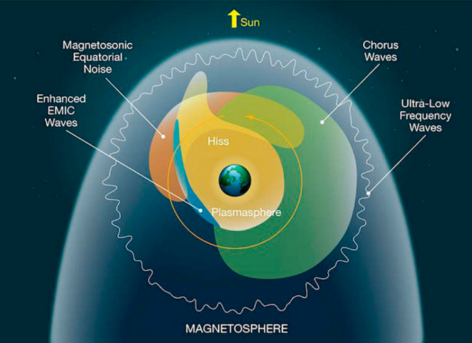
Lower hybrid waves: ???
Whistler waves (Section 10.6)
Chorus waves
- 1-5 kHz (\(0.1-1.0\,f_{ce}\)), well-defined narrow band
- highly nonlinear
- not generated by lightning, but by natural plasma instabilities (same for hiss).
- electron anisotropy
- loss cone scattering
Hiss waves
- broadband structureless signal in the plasmasphere and resembles audible hiss

Before 1990s, waves in the radiation belts are known for transferring energy from charged particles, which act as a loss process to the particles. Richard Thorne, together with his collegues, proposed that they could also the sources of energetic particles ([Horne & Thorne], 1998, 2003, 2005a,b). If that is the case, the wave-particle interactions must break the adiabatic invariants.
The theory of wave-particle interaction starts with hot plasma kinetic theory (Section 12.10.1). When the denominator goes to 0, the resonance condition is fulfilled. From observations, we learned that the wave frequencies are smaller than the gyro-frequencies. How can we have resonance then? The answer is, Doppler shift needs to be taken into account.
24.1.1 Sources of Waves
resonance can generate current => this current can generate higher frequency radiations?
Whistler waves can be explained by the linear theory. However, chorus and hiss waves are highly nonlinear and thus cannot be explained by a linear theory. We conjecture that they are caused by natural plasma instabilities, but we still have little idea what exactly these instabilities are.
As a rough physical picture, during the cyclotron resonance:
- Waves diffuse source electrons into loss cone => electron loss and wave growth.
- Waves diffuse trapped electrons => energy diffusion leads to electron acceleration.
24.2 Modeling
3D Fokker-Planck diffusion model1 (e.g. (Glauert et al. 2014)) has been built to model the radiation belt electrons. In the Earth’s radiation belts, the evolution of the phase-averaged phase-space density \(f(p,r,t)\) can be described by a diffusion equation (see also Equation 12.19): \[ \frac{\partial f}{\partial t} = \sum_{i,j}\frac{\partial}{\partial J_i}\left[ D_{ij}\frac{\partial f}{\partial J_j} \right] \tag{24.1}\]
Here \(D_{ij}\) are diffusion coefficients and \(J_i\) are the action integrals, \(J_1 = 2\pi m_e \mu/|q|\), \(J_2 = J\), and \(J_3 = q|\phi|\), where \(\mu,J\), and \(\phi\) are the adiabatic invariants of charged particle motion, \(m_e\) is the electron mass, and \(q\) the charge. The adiabatic invariants are awkward variables to visualize and relate to data so many authors transform to other coordinates. One choice is to use pitch angle, energy, and \(L^\ast=2\pi M/(|\phi| R_\text{E})\) (Equation 7.48), where \(M=8.22\times 10^{22}\, \text{A}\,\text{m}^2\) is the magnetic moment of the Earth’s dipole field and \(R_\text{E}\) is the Earth’s radius, as the three independent variables.
Assuming a dipole field, changing coordinates to equatorial pitch angle \(\alpha\), kinetic energy \(E\), and \(L^\ast\), and neglecting some cross derivatives, Equation 12.19 can be written as \[ \begin{aligned} \frac{\partial f}{\partial t} =& \frac{1}{g(\alpha)}\frac{\partial}{\partial \alpha}\bigg\rvert_{E,L} g(\alpha)\left( D_{\alpha\alpha}\frac{\partial f}{\partial\alpha}\bigg\rvert_{E,L} + D_{\alpha E}\frac{\partial f}{\partial E}\bigg\rvert_{\alpha,L} \right) \\ &+ \frac{1}{A(E)}\frac{\partial}{\partial E}\bigg\rvert_{\alpha,L} A(E) \left( D_{EE}\frac{\partial f}{\partial E}\bigg\rvert_{\alpha,L} + D_{E\alpha}\frac{\partial f}{\partial \alpha}\bigg\rvert_{E,L} \right) \\ &+ L^2 \frac{\partial}{\partial L}\bigg\rvert_{\mu,J}\left( \frac{D_{LL}}{L^2}\frac{\partial f}{\partial L}\bigg\rvert_{\mu,J} \right) \end{aligned} \tag{24.2}\] where \[ \begin{aligned} g(\alpha) = T(\alpha)\sin 2\alpha \\ A(E) = (E+E_0)(E(E+2E_0))^{1/2} \end{aligned} \] and \(E_0\) is the electron rest mass energy. \(T(\alpha)\) is related to the bounce period and in a dipole field can be approximated by \[ T(\alpha) = \big(1.3802 - 0.3198(\sin\alpha + \sin^{1/2} \alpha) \big) \]
\(D_{\alpha\alpha},\, D_{\alpha E}=D_{E\alpha},\, D_{EE}\), and \(D_{LL}\) are the drift- and bounce-averaged pitch angle, mixed pitch angle energy, energy and radial diffusion coefficients, respectively. When we need to clarify the fact that they are drift and bounce averaged, they will be explicitly written as \(\left< D_{\alpha\alpha} \right>^d, \left< D_{\alpha E} \right>^d, \left< D_{EE} \right>^d\), and \(\left< D_{LL} \right>^d\), respectively.
The bounce-averaged pitch angle and energy diffusion rates are defined by \[ \begin{aligned} \left< D_{\alpha\alpha} \right> &\equiv \left< \frac{(\Delta\alpha)^2}{2\Delta t} \right> \\ \left< D_{\alpha E} \right> &\equiv \left< \frac{(\Delta\alpha \Delta E)^2}{2\Delta t} \right> \\ \left< D_{EE} \right> &\equiv \left< \frac{(\Delta E)^2}{2\Delta t} \right> \end{aligned} \] with units of \(\text{s}^{-1}, \text{J}\text{s}^{-1}\), and \(\text{J}^2\text{s}^{-1}\), respectively.
A loss term of the form \(f/\tau_L\) can be added to represent losses to the atmosphere due to collisions. Here, \(\tau_L\), the loss timescale, is equal to 1/4 of the bounce time in the loss cone and infinite elsewhere. As a first-order approximation, we can neglect the cross terms and simplify Equation 24.2 as \[ \begin{aligned} \frac{\partial f}{\partial t} =& \frac{1}{g(\alpha)}\frac{\partial}{\partial \alpha}\bigg\rvert_{E,L} g(\alpha)\left( D_{\alpha\alpha}\frac{\partial f}{\partial\alpha}\bigg\rvert_{E,L}\right) \\ &+ \frac{1}{A(E)}\frac{\partial}{\partial E}\bigg\rvert_{\alpha,L} A(E) \left( D_{EE}\frac{\partial f}{\partial E}\bigg\rvert_{\alpha,L}\right) \\ &+ L^2 \frac{\partial}{\partial L}\bigg\rvert_{\mu,J}\left( \frac{D_{LL}}{L^2}\frac{\partial f}{\partial L}\bigg\rvert_{\mu,J} \right) \\ &- \frac{f}{\tau_L} \end{aligned} \tag{24.3}\]
The first three terms on the right-hand side represent pitch angle, energy, and radial diffusion, respectively. The final term accounts for losses to the atmosphere. Pitch angle diffusion has contributions from wave-particle interactions and Coulomb collisions with the atmosphere, though the latter are only significant inside the loss cone. Energy diffusion is due to wave-particle interactions and radial diffusion to interactions with large-scale fluctuations in the Earth’s magnetic and electric fields. The diffusion coefficients are based on statistical wave models derived from data. Depending on the choice of the diffusion coefficients, the Fokker-Planck equation can be linear, quasi-linear, or nonlinear.
Let us make our lives even simpler by considering only the radial diffusion and loss term. The quasi-linear assumptions are:
- Broadband wave spectrum (with random phase), typically assumed as a Gaussian centered around a single dominant mode
- Low amplitude fluctuations (no nonlinear interactions)
- “Resonance limit” (linear growth rate of instabilities goes to 0)
- ULF wave-particle interactions lumped into the diffusion coefficient
Even when quasi-linear theory works fine, there are multiple sources of uncertainties in the radial diffusion coefficient:
- Background magnetic field model
- Bounce + drift average eliminates MLT dependence
- Azimuthal wave structure (i.e. power distribution over mode numbers)
Given the limited observation data, we want to estimate the unknown parameters \(D_{LL}, \tau_L\). This is called an inverse problem. In 2000, Brautigam and Albert proposed a dependence of the radial diffusion coefficent on \(K_p\) and L: \[ D_{LL} \approx 10^{-0.506 K_p(t) - 9.325}L^10 \]
The standard statistical approach is to apply a Bayesian parameter estimation, where we are looking for a distribution of parameters and correcting results based on new observations. However, it is difficult to apply in high dimensions, which typically requires the Markov-chain Monte Carlo (MCMC) approach. For example, our assumption is that the parameters can be written in the following forms: \[ \begin{aligned} D_{LL}(L, t) &= 10^(a K_p(t) + b)L^c \\ \tau_L(L, t) &= \left\{ \begin{array}{lr} (a_0 + a_1 L + a_2 L^2) / K_p(t) & \text{for } L\le L_{pp} \\ a_3 / K_p(t) & \text{for } L > L_{pp} \end{array} \right. \end{aligned} \] where \(L_{pp}\) is the plasmapause location, which can be estimated with some approximations. We introduce a bunch of random variables, and the posterior distributions of these variables after MCMC give us the best fits.
A new trend is to use physics-informed machine learning to learn the coefficients. First we may need to constrain the forms of the coefficients to avoid an ill-posed inverse problem. Let the physical loss term be described by a drift coefficient \(C\): \[ \frac{\partial f}{\partial t} = L^2 \frac{\partial}{\partial L}\bigg\rvert_{\mu,J}\left( \frac{D_{LL}}{L^2}\frac{\partial f}{\partial L}\bigg\rvert_{\mu,J} \right) - \frac{\partial Cf}{\partial L} \]
The job of Physical-Informed Neural Network (PINN) is to deduce the optimal \(D_{LL}\) and \(C\) based on statistics by embedding the expected form of the equation into the loss term in the neural network. As this is statistics, we can build and test any kind of relations between variables without physical interpretation, which has been critizised a lot. For example, one may ask how you can let the phase space distribution \(f\) depend only on \(t\) and \(L\)? The information is incomplete from a physics point of view, but datawise it may just “work”, in the sense that neural network is essentially a universal high-dimensional function approximator.
24.2.1 Coupling physical processes at different time scales
If we only look at low frequency regime, the high frequency wave-particle interactions behave as a diffusion process to the plasma. Thus the coupling idea is not to simulate everything on the same time scale, but simulate the radiation belt effect by macroscopic diffusion coefficients.
24.3 Loss
Quantitative understanding of the electron acceleration mechanisms falls short, mostly due to the lack of understanding of the loss mechanisms.
- Bounce loss cone
- Drift loss cone
24.4 Plasmasphere
The plasmasphere is a region within the Earth’s magnetosphere that contains dense, cold plasma. It is located in the innermost part of the magnetosphere, and it extends from about 1,000 to 60,000 kilometers above the Earth’s surface. The plasmasphere is formed by the Earth’s magnetic field, which traps charged particles in the region, creating a donut-shaped structure around the planet.

The plasma in the plasmasphere is composed mainly of ions and electrons, and it is much colder and denser than the plasma in other regions of the magnetosphere.
- \(T \in [10^3, 10^4]\,\mathrm{K}\)
- \(N \in [10^1, 10^2]\,\mathrm{cm}^{-3}\)
The plasmasphere plays an important role in the dynamics of the Earth’s magnetosphere and its interactions with the solar wind. It can affect the propagation of radio waves, particularly those used for communication and navigation, and it can also contribute to the formation of the aurora borealis and aurora australis.
The general form of the Fokker-Planck equation also includes an advection term, which is ignored here since the drift is negligible compared to diffusion.↩︎