Guiding Center Approximation
This example demonstrates how to solve the guiding center (GC) equations directly. More theoretical details can be found in Guiding Center.
using TestParticle, OrdinaryDiffEq, StaticArrays
import TestParticle as TP
using Statistics: median, norm
using CairoMakie, Chairmarks
using DiffEqCallbacks
Curved B Field
First, we demonstrate the motion in a curved magnetic field. The magnetic field satisfies
function curved_B(x)
    # satisify ∇ ⋅ B = 0
    # B_θ = 1/r => ∂B_θ/∂θ = 0
    θ = atan(x[3] / (x[1] + 3))
    r = sqrt((x[1] + 3)^2 + x[3]^2)
    return SA[-1.0e-6 * sin(θ) / r, 0, 1.0e-6 * cos(θ) / r]
end

uniform_B(x) = SA[0.0, 0.0, 1.0e-8]
uniform_E(x) = SA[1.0e-9, 0.0, 0.0]

# Initial condition
stateinit = let x0 = [1.0, 0, 0], v0 = [0.0, 1.0, 0.1]
    [x0..., v0...]
end
# Time span
tspan = (0, 41)

# 1. Full Orbit Simulation
param = prepare(uniform_E, curved_B, species = Proton)
prob = ODEProblem(trace!, stateinit, tspan, param)
sol = solve(prob, Vern9())

# 2. Guiding Center Simulations
stateinit_gc, param_gc = TP.prepare_gc(
    stateinit, uniform_E, curved_B,
    species = Proton
)
prob_gc = ODEProblem(trace_gc!, stateinit_gc, tspan, param_gc)
sol_gc = solve(prob_gc, Vern9())

# Native GC Solvers
prob_native = TraceGCProblem(stateinit_gc, tspan, param_gc)
sol_native_rk4 = TP.solve(prob_native; dt = 0.1, alg = :rk4).u[1]
sol_native_rk45 = TP.solve(prob_native; alg = :rk45).u[1]

# Guiding Center Simulation with Numeric B Field Interpolation
xrange = range(0.9, 1.2, length = 20)
yrange = range(-0.5, 0.1, length = 60)
zrange = range(-0.8, 0.8, length = 40)

B_numerical = Array{Float64, 4}(undef, 3, length(xrange), length(yrange), length(zrange))
for k in eachindex(zrange), j in eachindex(yrange), i in eachindex(xrange)
    x = SA[xrange[i], yrange[j], zrange[k]]
    B_numerical[:, i, j, k] = curved_B(x)
end

stateinit_gc_num, param_gc_num = TP.prepare_gc(
    stateinit, xrange, yrange, zrange,
    uniform_E, B_numerical, species = Proton, order = 3
)

prob_gc_num = ODEProblem(trace_gc!, stateinit_gc_num, tspan, param_gc_num)
sol_gc_numericBfield = solve(prob_gc_num, Vern9())

# 3. Analytic Guiding Center Drift
gc = param |> get_gc_func
gc_x0 = gc(stateinit) |> Vector
prob_gc_analytic = ODEProblem(trace_gc_drifts!, gc_x0, tspan, (param..., sol))
sol_gc_analytic = solve(prob_gc_analytic, Vern9(); save_idxs = [1, 2, 3])

# 4. GC Simulation with Velocity Saving
# Save the perpendicular velocities on-the-fly.
saved_values = SavedValues(Float64, SVector{3, Float64})
# The callback function must use the form `save_func(u, t, integrator)`
# where `integrator.p` holds the parameters.
cb = SavingCallback((u, t, integrator) -> get_gc_velocity(u, integrator.p, t), saved_values)

# Reuse the parameters from the previous GC simulation
prob_gc_saving = ODEProblem(trace_gc!, stateinit_gc, tspan, param_gc)
sol_gc_saving = solve(prob_gc_saving, Vern9(), callback = cb)

# 5. Trace Magnetic Field Lines
# Trace from the initial position and a few neighbors to show topology
b_lines = ODESolution[]
for dz in -0.2:0.1:0.2
    u0 = stateinit[1:3] + [0, 0, dz]
    prob_fl = TraceFieldlineProblem(u0, curved_B, (0.0, 3.0), mode = :both)
    push!(b_lines, solve(prob_fl[1], Tsit5()))
    push!(b_lines, solve(prob_fl[2], Tsit5()))
end

# Visualization
f = Figure(size = (1000, 800), fontsize = 18)

# Left Panel: 3D Trajectory
ax1 = Axis3(
    f[1, 1],
    title = "3D Trajectories",
    xlabel = "x [m]",
    ylabel = "y [m]",
    zlabel = "z [m]",
    aspect = :data
)

# Right Panel: 2D Projection (X-Z plane)
ax2 = Axis(
    f[1, 2],
    title = "2D Projection (X-Z)",
    xlabel = "x [m]",
    ylabel = "z [m]",
    aspect = DataAspect()
)

# Plot Helper
gc_plot(x, y, z, vx, vy, vz) = (gc([x, y, z, vx, vy, vz])...,)
gc_plot_xz(x, y, z, vx, vy, vz) = (gc([x, y, z, vx, vy, vz])[[1, 3]]...,)

# Plot Field Lines
for bl in b_lines
    color = (:grey, 0.5)
    lines!(ax2, bl, idxs = (1, 3), color = color)
end

# Plot Trajectories
c1 = Makie.wong_colors()[1]
c2 = Makie.wong_colors()[2]
c3 = Makie.wong_colors()[3]
c4 = Makie.wong_colors()[4]
c5 = Makie.wong_colors()[5]

# 3D Plotting
lines!(ax1, sol, idxs = (1, 2, 3), color = (c1, 0.5), label = "Particle")
lines!(ax1, sol_gc, idxs = (1, 2, 3), color = c2, label = "GC (Trace)")
lines!(ax1, sol_native_rk4, idxs = (1, 2, 3), color = c2, linestyle = :dash, label = "Native GC (RK4)")
lines!(ax1, sol_native_rk45, idxs = (1, 2, 3), color = c2, linestyle = :dot, label = "Native GC (RK45)")
lines!(ax1, sol_gc_numericBfield, idxs = (1, 2, 3), color = c3, label = "GC (Numeric B)")
lines!(ax1, sol_gc_analytic, idxs = (1, 2, 3), color = c4, label = "GC (Analytic)")
lines!(
    ax1, sol, idxs = (gc_plot, 1, 2, 3, 4, 5, 6), color = c5, label = "GC (From Particle)"
)

# 2D Plotting
lines!(ax2, sol, idxs = (1, 3), color = (c1, 0.5))
lines!(ax2, sol_gc, idxs = (1, 3), color = c2)
lines!(ax2, sol_native_rk4, idxs = (1, 3), color = c2, linestyle = :dash)
lines!(ax2, sol_native_rk45, idxs = (1, 3), color = c2, linestyle = :dot)
lines!(ax2, sol_gc_numericBfield, idxs = (1, 3), color = c3)
lines!(ax2, sol_gc_analytic, idxs = (1, 3), color = c4)
lines!(ax2, sol, idxs = (gc_plot_xz, 1, 2, 3, 4, 5, 6), color = c5)

axislegend(ax1, position = :rt, backgroundcolor = :transparent)

# Error Analysis (Relative to Analytic GC)
ts = range(tspan..., length = 100)
gc_ref = sol_gc_analytic(ts)

# 1. Trace GC Error
gc_trace = sol_gc(ts)
err_trace = [norm(u[1:3] - v) for (u, v) in zip(gc_trace.u, gc_ref.u)]

# 2. Numeric B GC Error
gc_num = sol_gc_numericBfield(ts)
err_num = [norm(u[1:3] - v) for (u, v) in zip(gc_num.u, gc_ref.u)]

# 3. GC from Particle Error
gc_part = [gc([sol(t)...]) for t in ts]
err_part = [norm(u - v) for (u, v) in zip(gc_part, gc_ref.u)]

ax3 = Axis(
    f[2, 1:2],
    title = "Deviation from Analytic Guiding Center",
    xlabel = "Time [s]",
    ylabel = "Distance [m]",
    yscale = log10
)

lines!(ax3, ts, err_trace, color = c2, label = "Trace GC")
lines!(ax3, ts, err_num, color = c3, label = "Numeric B GC")
lines!(ax3, ts, err_part, color = c5, label = "GC from Particle")

axislegend(ax3, position = :rt, backgroundcolor = :transparent)
rowsize!(f.layout, 1, Relative(3 / 4))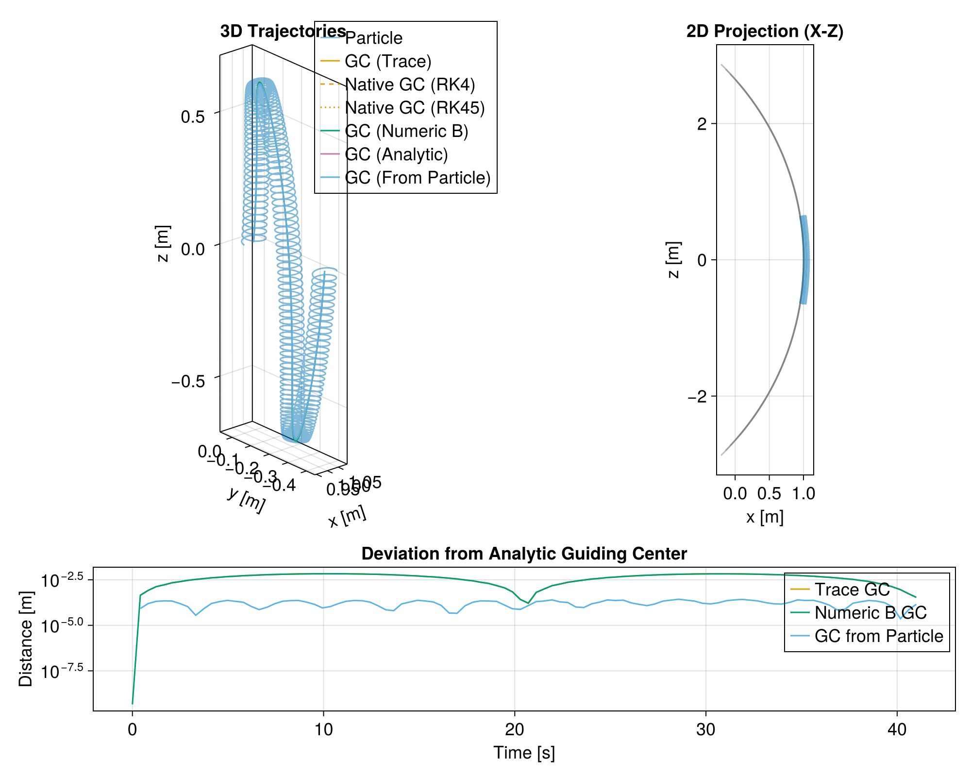
Scale Comparison (Grad-B Drift)
It is important to satisfy the strict scale requirements for the GC approximation. The gyro-radius must be much smaller than the characteristic spatial scales of the EM fields for the finite-Larmor-radius (FLR) 1st order approximation to be valid.
We compare two cases: 2. Large Radius: Weaker magnetic field, larger gyroradius.
- Small Radius: Stronger magnetic field, smaller gyroradius.
function run_grad_B_sim(B_func, tspan)
    # Particle
    param = prepare(uniform_E, B_func, species = Proton)
    prob = ODEProblem(trace!, stateinit, tspan, param)
    sol = solve(prob, Vern9())

    # GC (Trace)
    stateinit_gc,
        param_gc = TP.prepare_gc(
        stateinit, uniform_E, B_func,
        species = Proton
    )
    prob_gc = ODEProblem(trace_gc!, stateinit_gc, tspan, param_gc)
    sol_gc = solve(prob_gc, Vern9())

    # GC (Analytic)
    gc = param |> get_gc_func
    gc_x0 = gc(stateinit) |> Vector
    prob_gc_analytic = ODEProblem(trace_gc_drifts!, gc_x0, tspan, (param..., sol))
    sol_gc_analytic = solve(prob_gc_analytic, Vern9(); save_idxs = [1, 2, 3])

    # GC from Particle
    gc_from_particle = (sol, gc)

    return sol, sol_gc, sol_gc_analytic, gc_from_particle
end

# Case 1: Large radius
grad_B_large(x) = SA[0, 0, 1.0e-8 + 1.0e-9 * x[2]]
tspan_large = (0, 20)
results_large = run_grad_B_sim(grad_B_large, tspan_large)

# Case 2: Small radius
grad_B_small(x) = SA[0, 0, 1.0e-7 + 1.0e-8 * x[2]]
tspan_small = (0, 10)
results_small = run_grad_B_sim(grad_B_small, tspan_small)

# Visualization
f2 = Figure(size = (1000, 500), fontsize = 18)

function plot_results!(ax, res, title_str)
    sol, sol_gc, sol_gc_analytic, (sol_p, gc_func) = res

    # Helper for GC from Particle
    gc_plot(x, y, z, vx, vy, vz) = (gc_func([x, y, z, vx, vy, vz])...,)

    lines!(ax, sol, idxs = (1, 2, 3), color = (c1, 0.4), label = "Particle")
    lines!(ax, sol_gc, idxs = (1, 2, 3), color = c2, label = "GC (Trace)")
    lines!(ax, sol_gc_analytic, idxs = (1, 2, 3), color = c4, label = "GC (Analytic)")
    lines!(
        ax, sol_p, idxs = (gc_plot, 1, 2, 3, 4, 5, 6),
        color = c5, label = "GC (From Particle)"
    )

    ax.title = title_str
    ax.xlabel = "x [m]"
    ax.ylabel = "y [m]"
    ax.zlabel = "z [m]"
    return ax.aspect = :data
end

ax_left = Axis3(f2[1, 1])
plot_results!(ax_left, results_large, "Weak B")

ax_right = Axis3(f2[1, 2])
plot_results!(ax_right, results_small, "Strong B")

axislegend(ax_left, backgroundcolor = :transparent)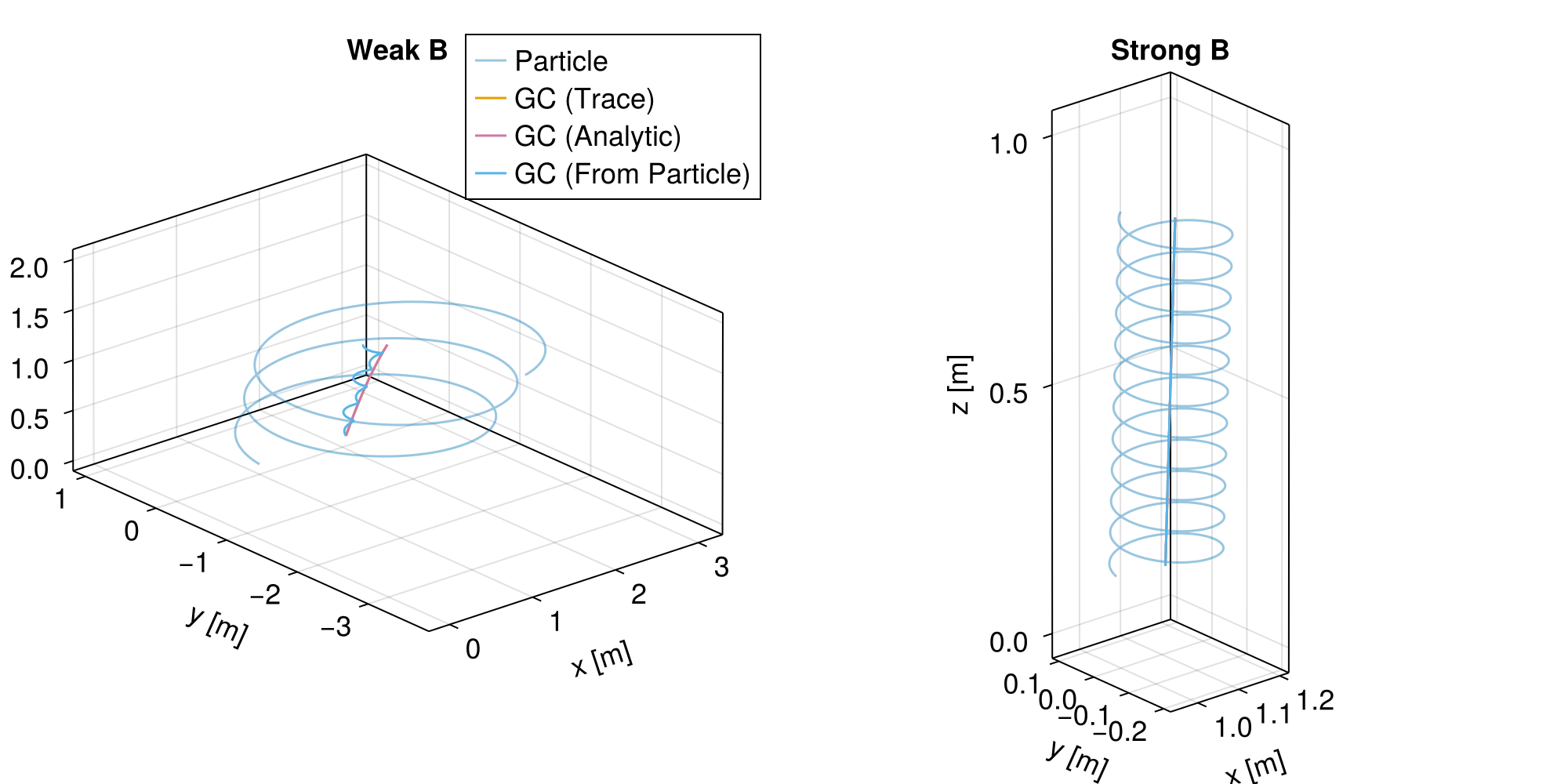
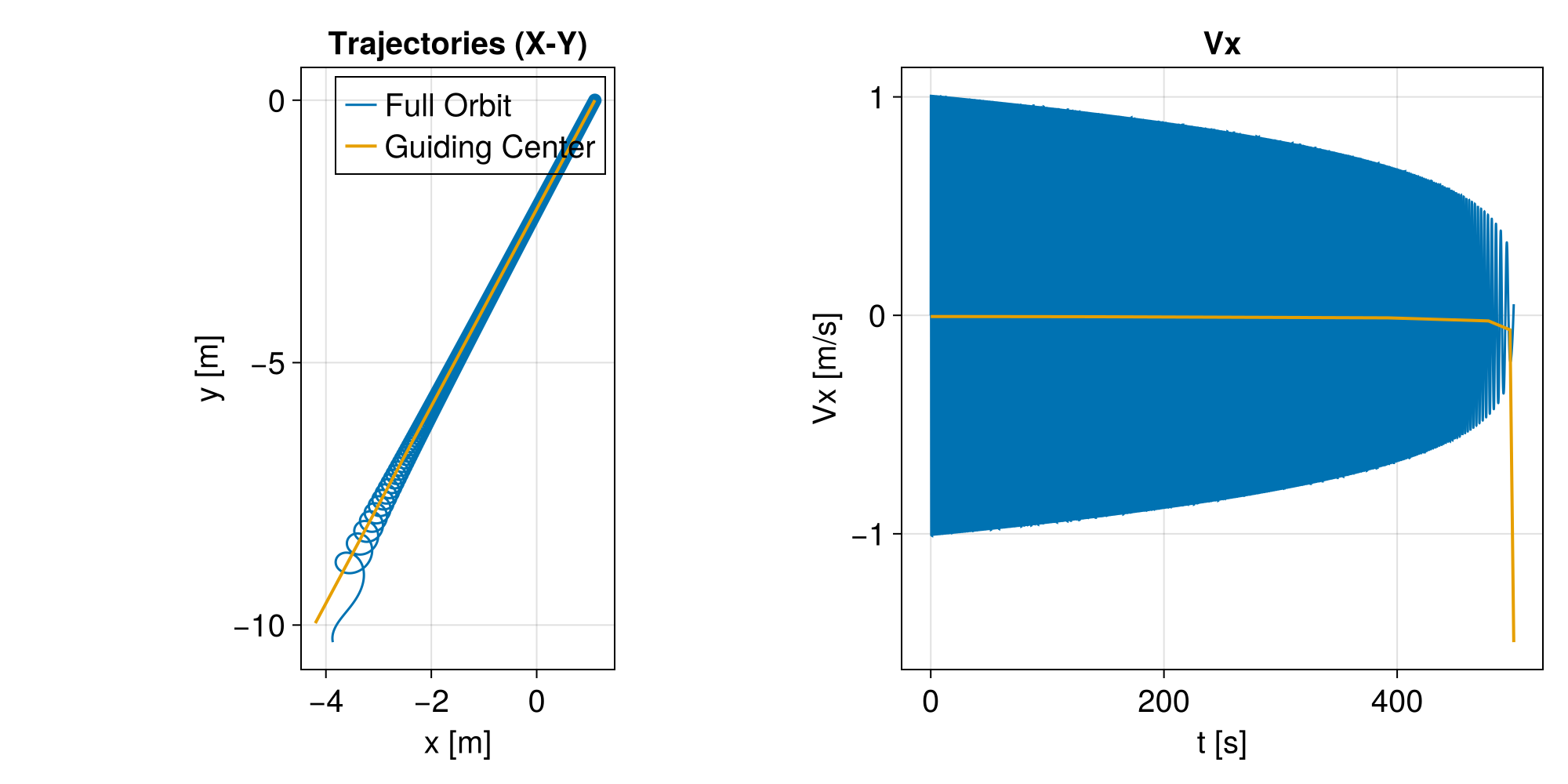
Performance Comparison
The Guiding Center approximation allows for much larger time steps because it averages out the rapid gyromotion. This results in significant performance gains, especially for long-term simulations in strong magnetic fields.
# Prepare longer simulation for benchmark
tspan_bench = (0, 500.0)

# Full Particle Problem
param_full = prepare(uniform_E, grad_B_small, species = Proton)
prob_full = ODEProblem(trace!, stateinit, tspan_bench, param_full)

# Guiding Center Problem
stateinit_gc,
    param_gc = TP.prepare_gc(
    stateinit, uniform_E, grad_B_small,
    species = Proton
)
# Save the perpendicular velocities on-the-fly.
saved_values = SavedValues(Float64, SVector{3, Float64})
cb = SavingCallback(
    (u, t, integrator) -> get_gc_velocity(u, integrator.p, t), saved_values
)
prob_gc = ODEProblem(trace_gc!, stateinit_gc, tspan_bench, param_gc)

# Native GC Problem
prob_native_gc = TraceGCProblem(stateinit_gc, tspan_bench, param_gc)

# Run simulations for plotting
sol_full = solve(prob_full, Vern9())
sol_gc_trace = solve(prob_gc, Vern9(), callback = cb)

# Benchmark
b_full = @be solve(prob_full, Vern9())
b_gc = @be solve(prob_gc, Vern9())
b_native_rk4 = @be TP.solve(prob_native_gc; dt = 1.0, alg = :rk4)
b_native_rk45 = @be TP.solve(prob_native_gc; alg = :rk45)

# Visualization of Benchmark Results
f3 = Figure(size = (1000, 500), fontsize = 20)

# Left Panel: Trajectories (X-Y plane)
ax_traj = Axis(
    f3[1, 1],
    title = "Trajectories (X-Y)",
    xlabel = "x [m]",
    ylabel = "y [m]",
    aspect = DataAspect()
)

lines!(ax_traj, sol_full, idxs = (1, 2), color = c1, label = "Full Orbit")
lines!(
    ax_traj, sol_gc_trace, idxs = (1, 2), color = c2,
    linewidth = 2, label = "Guiding Center"
)
axislegend(ax_traj, backgroundcolor = :transparent)

# Right Panel: Vx
ax_vel = Axis(
    f3[1, 2],
    title = "Vx",
    xlabel = "t [s]",
    ylabel = "Vx [m/s]"
)

lines!(ax_vel, sol_full, idxs = (4), color = c1, label = "Full Orbit")
lines!(
    ax_vel, saved_values.t, [v[1] for v in saved_values.saveval],
    color = c2, linewidth = 2, label = "Guiding Center"
)
Performance
| Solver | Time | Memory | Ratio |
|---|---|---|---|
| Full Orbit | 0.00166 | 2.9e6 | 1.0 |
| Guiding Center | 2.02e-5 | 18600.0 | 0.0122 |
| Native GC (RK4) | 0.000118 | 20600.0 | 0.0711 |
| Native GC (RK45) | 4.38e-5 | 8020.0 | 0.0264 |