Magnetic Dipole

This example shows how to trace protons of a certain energy in a analytic Earth-like magnetic dipole field. There is a combination of grad-B drift, curvature drift, and the bounce motion between mirror points. It demonstrates the motions corresponding to the three adiabatic invariants.

julia

using TestParticle, OrdinaryDiffEq
import TestParticle as TP
using TestParticle: mᵢ, qᵢ, c, Rₑ
using CairoMakie

# Initial condition
stateinit = let
   # Initial particle energy
   Ek = 5e7 # [eV]
   # initial velocity, [m/s]
   v₀ = TP.sph2cart(c*sqrt(1-1/(1+Ek*qᵢ/(mᵢ*c^2))^2), π/4, 0.0)
   # initial position, [m]
   r₀ = TP.sph2cart(2.5*Rₑ, π/2, 0.0)
   [r₀..., v₀...]
end
# obtain field
param = prepare(TP.DipoleField())
tspan = (0.0, 10.0)

prob = ODEProblem(trace!, stateinit, tspan, param)

sol = solve(prob, Vern9())

### Visualization

f = Figure(fontsize = 18)
ax = Axis3(f[1, 1],
   title = "50 MeV Proton trajectory in Earth's dipole field",
   xlabel = "x [Re]",
   ylabel = "y [Re]",
   zlabel = "z [Re]",
   aspect = :data,
   limits = (-2.5, 2.5, -2.5, 2.5, -1, 1)
)

x = sol[1, :] ./ Rₑ
y = sol[2, :] ./ Rₑ
z = sol[3, :] ./ Rₑ
lines!(ax, x, y, z)

for ϕ in range(0, stop = 2*π, length = 10)
   lines!(ax, TP.dipole_fieldline(ϕ)..., color = :tomato, alpha = 0.3)
end

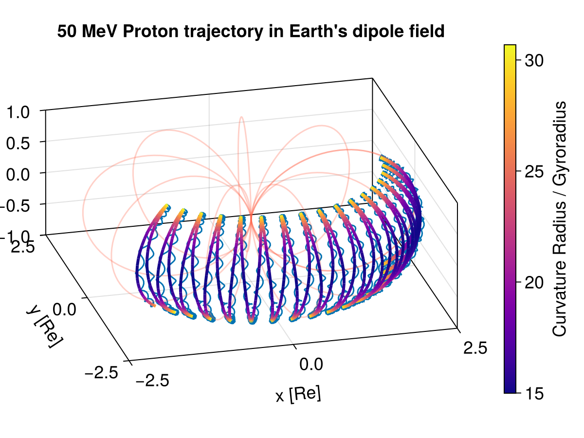
Solver algorithm matters in terms of energy conservation. In the above we used Verner's “Most Efficient” 9/8 Runge-Kutta method. Let's check other algorithms.

julia

function get_energy_ratio(sol)
   vx = @view sol[4, :]
   vy = @view sol[5, :]
   vz = @view sol[6, :]

   Einit = vx[1]^2 + vy[1]^2 + vz[1]^2
   Eend = vx[end]^2 + vy[end]^2 + vz[end]^2

   (Eend - Einit) / Einit
end

using Markdown
using Printf

results = Tuple{String, Float64}[]

# OrdinaryDiffEq solvers
ode_solvers = [
   ("ImplicitMidpoint, dt=1e-3", ImplicitMidpoint(), Dict(:dt => 1e-3)),
   ("ImplicitMidpoint, dt=1e-4", ImplicitMidpoint(), Dict(:dt => 1e-4)),
   ("Vern9", Vern9(), Dict()),
   ("Trapezoid", Trapezoid(), Dict()),
   ("Vern6", Vern6(), Dict()),
   ("Tsit5", Tsit5(), Dict()),
   # Default stepsize settings may not be enough for our problem. By using a smaller `abstol` and `reltol`, we can guarantee much better conservation at a higher cost:
   # This is roughly equivalent in accuracy and performance with Vern9() and `reltol=1e-3` (default)
   ("Tsit5, reltol=1e-4", Tsit5(), Dict(:reltol => 1e-4))
]

for (name, alg, kwargs) in ode_solvers
   local sol = solve(prob, alg; kwargs...)
   push!(results, (name, get_energy_ratio(sol)))
end

Or, for adaptive time step algorithms like Vern9(), with the help of callbacks, we can enforce a largest time step smaller than 1/10 of the local gyroperiod:

julia

using DiffEqCallbacks

# p = (charge_mass_ratio, m, E, B)
dtFE(u, p, t) = 2π / (abs(p[1]) * sqrt(sum(x -> x^2, p[4](u, t))))

cb = StepsizeLimiter(dtFE; safety_factor = 1 // 10, max_step = true)

sol = solve(prob, Vern9(); callback = cb, dt = 0.1) # dt=0.1 is a dummy value
push!(results, ("Vern9 with StepsizeLimiter", get_energy_ratio(sol)));

This is much more accurate, at the cost of more iterations. In terms of accuracy, this is roughly equivalent to solve(prob, Vern9(); reltol=1e-7); in terms of performance, it is 2x slower (0.04s v.s. 0.02s) and consumes about the same amount of memory 42 MiB. We can also use the classical Boris method implemented within the package:

julia

dt = 1e-4
prob_boris = TraceProblem(stateinit, tspan, param)
sol_boris = TestParticle.solve(prob_boris; dt)[1]
push!(results, ("Boris method, dt=1e-4", get_energy_ratio(sol_boris)));

Comparison of energy conservation:

Solver	Energy Ratio
ImplicitMidpoint, dt=1e-3	-4.5982e-04
ImplicitMidpoint, dt=1e-4	-4.9401e-09
Vern9	-7.0779e-03
Trapezoid	-5.5139e-02
Vern6	-6.5781e-02
Tsit5	5.3520e-01
Tsit5, reltol=1e-4	6.3709e-03
Vern9 with StepsizeLimiter	-5.3994e-07
Boris method, dt=1e-4	-3.9618e-14

The Boris method requires a fixed time step. It takes about 0.05s and consumes 53 MiB memory. In this specific case, the time step is determined empirically. If we increase the time step to 1e-2 seconds, the trajectory becomes completely off (but the energy is still conserved). Therefore, as a rule of thumb, we should not use the default Tsit5() scheme without decreasing reltol. Use adaptive Vern9() for an unfamiliar field configuration, then switch to more accurate schemes if needed. A more thorough test can be found here.

Magnetic Dipole ​

Magnetic Dipole