Ensemble Tracing

This example demonstrates how to trace multiple particles efficiently using the EnsembleProblem interface from DifferentialEquations.jl. We cover three use cases:

1. Basic ensemble tracing with varying initial conditions.

2. Sampling initial velocities from a Maxwellian distribution.

3. Customizing output to save specific quantities (e.g., field values along trajectories).

4. Using the native Boris pusher for ensemble problems.

using TestParticle
import TestParticle as TP
using VelocityDistributionFunctions
using OrdinaryDiffEq
using StaticArrays
using Statistics
using LinearAlgebra
using Random
using CairoMakie

1. Basic Ensemble Tracing

In this section, we trace multiple electrons in a simple analytic EM field. We use prob_func to define unique initial conditions for each particle.

# Simulation parameters
B_analytic(x) = SA[0, 0, 1.0e-9]
E_analytic = ZeroField()
param = prepare(E_analytic, B_analytic, species = Electron)
tspan = (0.0, 10.0)
stateinit = SA[0.0, 0.0, 0.0, 1.0, 0.0, 0.0]
prob = ODEProblem(trace!, stateinit, tspan, param)

# Define prob_func to vary the initial x-velocity based on the particle index
prob_func_basic(prob, ctx) = remake(prob, u0 = [prob.u0[1:3]..., ctx.sim_id / 3, 0.0, 0.0])

trajectories = 3
ensemble_prob = EnsembleProblem(prob; prob_func = prob_func_basic, safetycopy = false)
sols = solve(ensemble_prob, Vern7(), EnsembleThreads(); trajectories)

# Visualization
f = Figure(fontsize = 20)
ax = Axis3(
    f[1, 1], title = "Basic Ensemble", xlabel = "X",
    ylabel = "Y", zlabel = "Z", aspect = :data
)

for (i, u) in enumerate(sols.u)
    lines!(ax, u[1, :], u[2, :], u[3, :]; label = "traj $i", color = Makie.wong_colors()[i])
end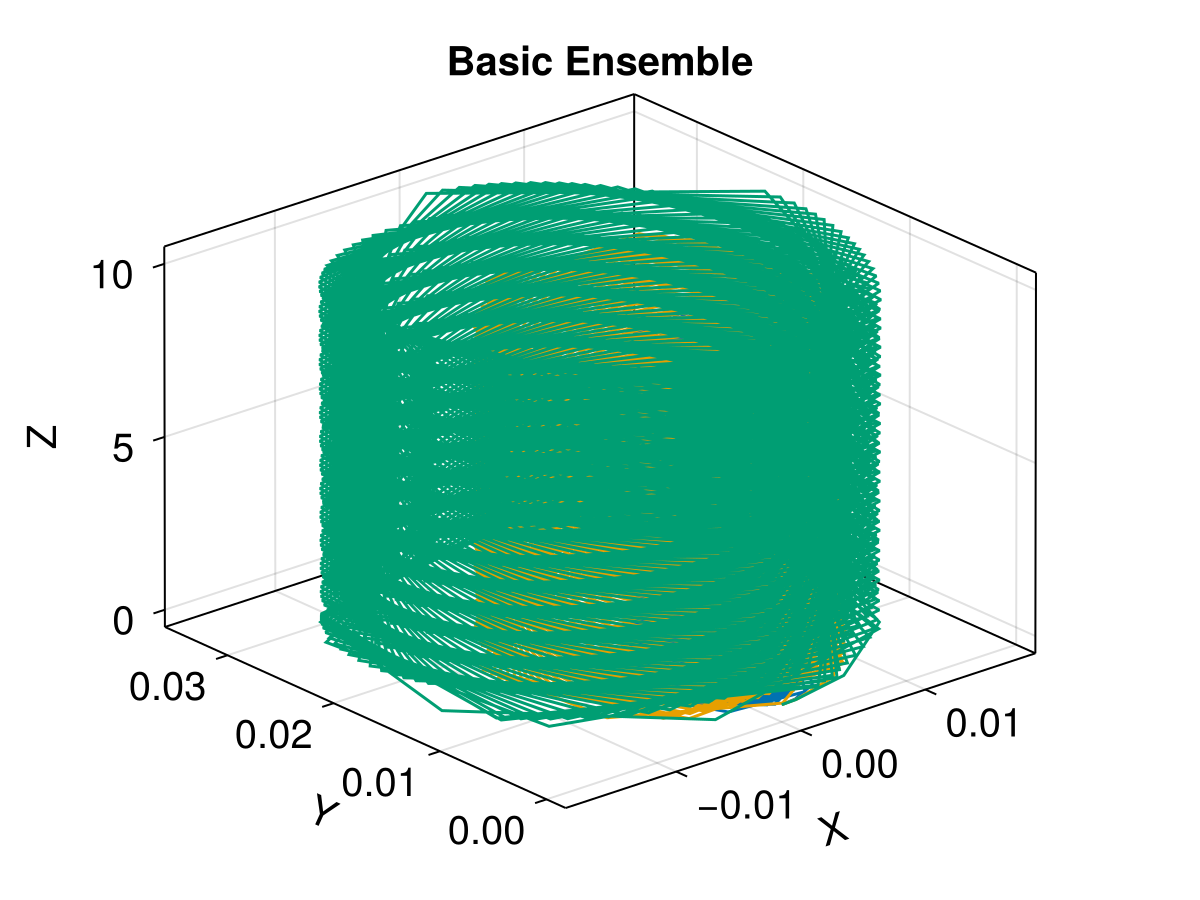

2. Sampling from a Distribution

Often we want to sample particle initial velocities from a distribution, such as a Maxwellian. Here we demonstrate how to do this using Maxwellian from TestParticle.jl.

Random.seed!(1234)

# Define a new prob_func that samples from a Maxwellian
function prob_func_maxwellian(prob, ctx)
    # Sample from a Maxwellian with bulk speed 0 and thermal speed 1.0
    vdf = TP.Maxwellian([0.0, 0.0, 0.0], 1.0)
    v = rand(vdf)
    return remake(prob; u0 = [prob.u0[1:3]..., v...])
end

trajectories_dist = 10
ensemble_prob_dist = EnsembleProblem(prob; prob_func = prob_func_maxwellian, safetycopy = false)
sols_dist = solve(ensemble_prob_dist, Vern7(), EnsembleThreads(); trajectories = trajectories_dist)

# Visualization
f = Figure(fontsize = 20)
ax = Axis3(
    f[1, 1], title = "Maxwellian Sampling", xlabel = "X",
    ylabel = "Y", zlabel = "Z", aspect = :data
)

for (i, u) in enumerate(sols_dist.u)
    lines!(ax, u[1, :], u[2, :], u[3, :], label = "$i", color = Makie.wong_colors()[mod1(i, 7)])
end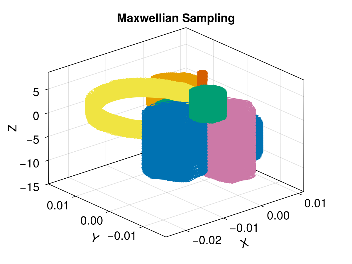

3. Customizing Output

Sometimes we don't need the entire trajectory, or we want to save additional data calculated during the simulation. The output_func allows us to customize what data is saved for each particle.

# Simulation parameters for custom output
B_analytic(x) = SA[0, 0, 1.0e-9]
E_analytic = ZeroField()
param_custom = prepare(E_analytic, B_analytic, species = Proton)
tspan_custom = (0.0, 40.0)
stateinit_custom = SA[0.0, 0.0, 0.0, 1.0, 0.0, 0.0]
prob_custom = ODEProblem(trace!, stateinit_custom, tspan_custom, param_custom)

# Define prob_func
function prob_func_custom(prob, ctx)
    return remake(prob, u0 = [stateinit_custom[1:3]..., 1.0, 0.0, Float64(ctx.sim_id)])
end

# Define output_func to save specific data
function output_func_custom(sol, i)
    getB = TP.get_BField(sol)
    b = getB.(sol.u)

    # Calculate cosine of pitch angle
    μ = [
        @views (b[j] ⋅ sol.u[j][4:6]) / (norm(b[j]) * norm(sol.u[j][4:6]))
            for j in eachindex(sol.u)
    ]

    # Return: (trajectory, B-field, pitch-angle-cosine), rerun_flag
    return (sol.u, b, μ), false
end

trajectories_custom = 2
saveat = tspan_custom[2] / 40

ensemble_prob_custom = EnsembleProblem(
    prob_custom;
    prob_func = prob_func_custom,
    output_func = output_func_custom,
    safetycopy = false
)

sols_custom = solve(
    ensemble_prob_custom, Vern9(), EnsembleThreads();
    trajectories = trajectories_custom,
    saveat = saveat
)

# Visualization
f = Figure(fontsize = 20)
ax = Axis3(
    f[1, 1], title = "Custom Output Trajectories",
    xlabel = "X", ylabel = "Y", zlabel = "Z", aspect = :data
)

for (i, u) in enumerate(sols_custom.u)
    # u[1] contains the trajectory (sol.u)
    traj = u[1]
    xp = [p[1] for p in traj]
    yp = [p[2] for p in traj]
    zp = [p[3] for p in traj]
    lines!(ax, xp, yp, zp, label = "traj $i", color = Makie.wong_colors()[i])
end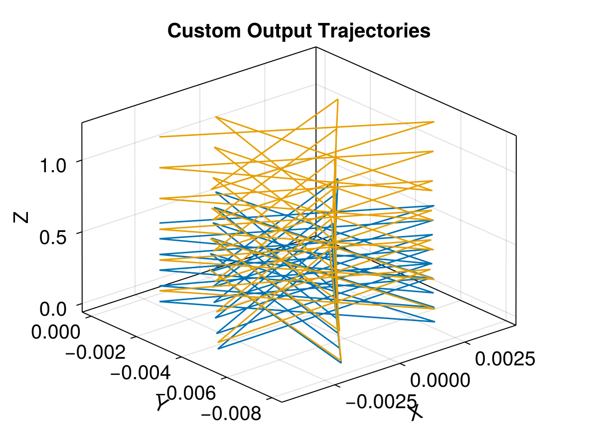

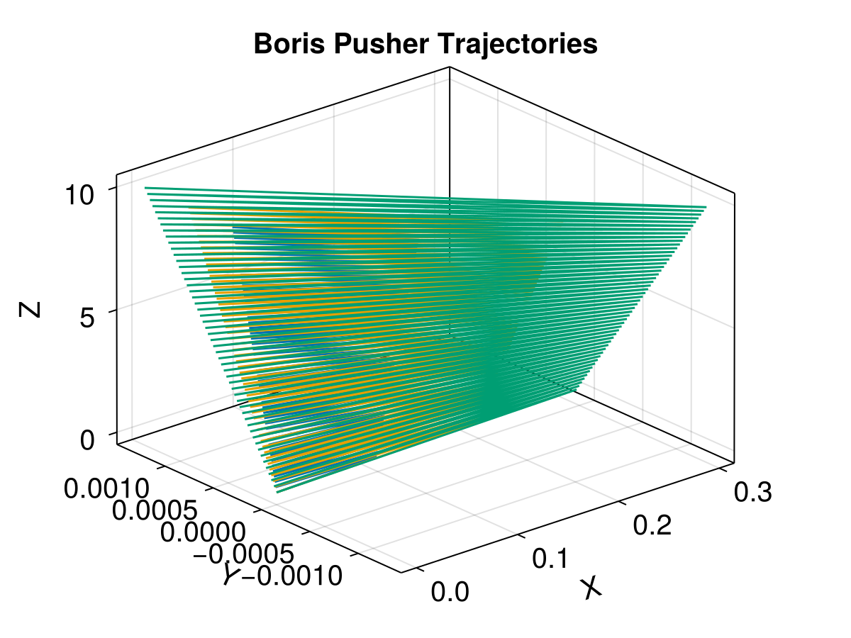
4. Native Boris Pusher

We can also solve the ensemble problem with the native Boris Method. Note that the Boris pusher requires additional parameters: a fixed timestep, and an output save interval.

dt = 0.1
savestepinterval = 1

# Reuse the basic problem parameters
prob_boris = TraceProblem(stateinit, tspan, param; prob_func = prob_func_basic)
trajs_boris = TestParticle.solve(prob_boris, Boris(); dt, trajectories = 3, savestepinterval)

# Visualization
f = Figure(fontsize = 20)
ax = Axis3(
    f[1, 1], title = "Boris Pusher Trajectories",
    xlabel = "X", ylabel = "Y", zlabel = "Z", aspect = :data
)

for (i, u) in enumerate(trajs_boris.u)
    lines!(ax, u[1, :], u[2, :], u[3, :], label = "$i", color = Makie.wong_colors()[i])
end