Analytical Magnetosphere

This demo shows how to trace particles in a comprehensive analytical model of the Earth's magnetosphere. The model is constructed using Magnetostatics.AnalyticalMagnetosphere, which incorporates an intrinsic dipole, a shielding dipole, a magnetotail (Harris sheet), and a uniform interplanetary magnetic field (IMF). In this model, magnetic null points appear, and the particle orbits are distorted from the idealized motions in Demo: magnetic dipole.

julia

using TestParticle, OrdinaryDiffEq, StaticArrays
using TestParticle: sph2cart, mᵢ, qᵢ, c, Rₑ, ZeroField
import Magnetostatics as MS
using FieldTracer
using CairoMakie

# Magnetosphere model parameters
R_MP = 10Rₑ
intrinsic_dipole = MS.Dipole(TestParticle.BMoment_Earth)
shielding_dipole = MS.Dipole(-TestParticle.BMoment_Earth)
shielding_dipole_pos = SA[2R_MP, 0.0, 0.0]

# Tail field parameters
Bt = 0.01 * 4.0e-5 # [T], 1% of the dipole field at the equator
δ = 0.1Rₑ # [m]
tail_field = MS.HarrisSheet(-Bt, δ)

# IMF
imf_field = MS.UniformField(SA[0.0, 0.0, -10.0e-9])

# Unified Analytical Magnetosphere model
mag_model = MS.AnalyticalMagnetosphere(;
    intrinsic_dipole,
    shielding_dipole,
    shielding_dipole_pos,
    tail_field,
    imf_field,
    mp_standoff = R_MP,
    bs_standoff = 14Rₑ,
    has_shock = true
)

@inbounds getB(r) = mag_model(SA[r[1], r[2], r[3]])

"""
Boundary condition check.
"""
function isoutside(u, p, t)
    rout = 18Rₑ
    return (u[1]^2 + u[2]^2 + u[3]^2) < (1.1Rₑ)^2 ||
        abs(u[1]) > rout || abs(u[2]) > rout || abs(u[3]) > rout
end

"""
Set initial conditions.
"""
function prob_func_13(prob, ctx)
    i = ctx.sim_id
    # initial particle energy
    Ek = 2.0e4 # [eV]
    # initial velocity, [m/s]
    v₀ = sph2cart(c * sqrt(1 - 1 / (1 + Ek * qᵢ / (mᵢ * c^2))^2), π / 4, 0.0)
    # initial position, [m]
    r₀ = sph2cart((10 - 2i) * Rₑ, π / 2, (i - 1.5) * π / 4)

    return prob = remake(prob; u0 = [r₀..., v₀...])
end

function prob_func_6(prob, ctx)
    i = ctx.sim_id
    # initial particle energy
    Ek = 4.0e3 # [eV]
    # initial velocity, [m/s]
    v₀ = sph2cart(c * sqrt(1 - 1 / (1 + Ek * qᵢ / (mᵢ * c^2))^2), π / 4, 0.0)
    # initial position, [m]
    r₀ = sph2cart(6 * Rₑ, π / 2, 2π * i)

    return prob = remake(prob; u0 = [r₀..., v₀...])
end

# obtain field
param = prepare(ZeroField(), getB)
stateinit = zeros(6) # particle position and velocity to be modified
tspan = (0.0, 2000.0)
trajectories = 2

prob = ODEProblem(trace!, stateinit, tspan, param)
ensemble_prob = EnsembleProblem(prob; prob_func = prob_func_13, safetycopy = false)

# See https://docs.sciml.ai/DiffEqDocs/stable/basics/common_solver_opts/
# for the solver options
callback = TerminateOutside(isoutside)
sols = solve(
    ensemble_prob, Vern7(), EnsembleSerial(); reltol = 1.0e-5,
    trajectories, callback, dense = true, save_on = true
)

### Visualization

f = Figure(fontsize = 20)
ax = Axis3(
    f[1, 1],
    title = "20 keV Protons in an analytical magnetosphere",
    xlabel = "x [Re]",
    ylabel = "y [Re]",
    zlabel = "z [Re]",
    aspect = :data,
    limits = (-8, 14, -10, 10, -5, 5),
    elevation = π / 6,
    azimuth = -π / 3
)

invRE = 1 / Rₑ

for (i, sol) in enumerate(sols.u)
    x = sol[1, :] .* invRE
    y = sol[2, :] .* invRE
    z = sol[3, :] .* invRE
    lines!(ax, x, y, z, color = Makie.wong_colors()[i])
end

# Field lines
function get_numerical_field(x, y, z, model)
    bx = zeros(length(x), length(y), length(z))
    by = similar(bx)
    bz = similar(bx)

    for i in CartesianIndices(bx)
        pos = SA[x[i[1]], y[i[2]], z[i[3]]]
        bx[i], by[i], bz[i] = model(pos)
    end

    return bx, by, bz
end

function trace_field!(
        ax, x, y, z, unitscale, model = getB;
        rmin = 4Rₑ, rmax = 16Rₑ, nr = 8, nϕ = 8
    )
    bx, by, bz = get_numerical_field(x, y, z, model)

    zs = 0.0
    dϕ = 2π / nϕ
    for r in range(rmin, rmax, length = nr), ϕ in range(0, 2π - dϕ, length = nϕ)
        xs = r * cos(ϕ)
        ys = r * sin(ϕ)
        x1, y1, z1 = FieldTracer.trace(
            bx, by, bz, xs, ys, zs, x, y, z;
            ds = 0.1Rₑ, maxstep = 10000
        )
        lines!(ax, x1 .* unitscale, y1 .* unitscale, z1 .* unitscale, color = :gray)
    end
    return
end

x = range(-8Rₑ, 14Rₑ, length = 50)
y = range(-10Rₑ, 10Rₑ, length = 50)
z = range(-8Rₑ, 8Rₑ, length = 50)

trace_field!(ax, x, y, z, invRE)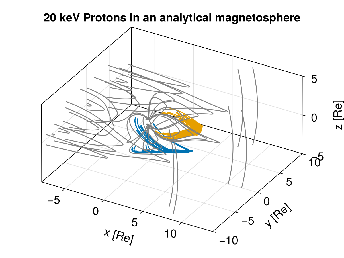

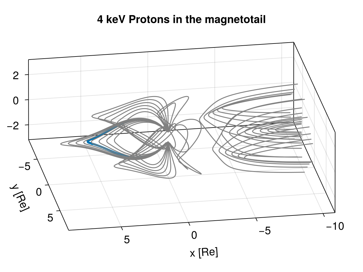
We now look at particles in the magnetotail region of the same model.

julia

param = prepare(ZeroField(), getB)
stateinit = zeros(6) # particle position and velocity to be modified
tspan = (0.0, 8000.0)
trajectories = 1

prob = ODEProblem(trace!, stateinit, tspan, param)
ensemble_prob = EnsembleProblem(prob; prob_func = prob_func_6, safetycopy = false)

callback = TerminateOutside(isoutside)
sols = solve(
    ensemble_prob, Vern9(), EnsembleSerial(); reltol = 1.0e-5,
    trajectories, callback, dense = true, save_on = true
)

x = range(-10Rₑ, 10Rₑ, length = 50)
y = range(-5Rₑ, 5Rₑ, length = 20)
z = range(-10Rₑ, 10Rₑ, length = 50)

f = Figure(fontsize = 18)
ax = Axis3(
    f[1, 1],
    title = "4 keV Protons in the magnetotail",
    xlabel = "x [Re]",
    ylabel = "y [Re]",
    zlabel = "z [Re]",
    aspect = :data,
    azimuth = 1.4
)

for (i, sol) in enumerate(sols.u)
    x_plot = sol[1, :] .* invRE
    y_plot = sol[2, :] .* invRE
    z_plot = sol[3, :] .* invRE
    lines!(ax, x_plot, y_plot, z_plot, color = Makie.wong_colors()[i])
end

trace_field!(ax, x, y, z, invRE, getB; rmin = 4Rₑ, rmax = 8Rₑ, nϕ = 8)

Analytical Magnetosphere ​

Analytical Magnetosphere