Shock Drift Acceleration at a Perpendicular Shock

This example shows Shock Drift Acceleration (SDA): a particle gains energy by drifting along the shock front in the convective electric field, while the cross-shock potential reflects it so it repeatedly hits the shock.

The setup is the perpendicular shock (${\theta }_{Bn}={90}^{\circ }$):

Quantity	Direction
Shock normal $\hat{\mathbf{n}}$	$+\hat{\mathbf{x}}$ (upstream $x<0$, downstream $x>0$)
Upstream flow ${\mathbf{V}}_1$	$+\hat{\mathbf{x}}$ (plasma flows into the shock)
Magnetic field ${\mathbf{B}}_1$	$+\hat{\mathbf{z}}$ (purely tangential)
Convection field $\mathbf{E}=-{\mathbf{V}}_1\times {\mathbf{B}}_1$	$+\hat{\mathbf{y}}$

The field only varies across the shock, so the only drift along the front is the gradient-$\mathbf{B}$ drift ${\mathbf{v}}_{\mathrm{\nabla }B}\propto (\mathbf{B}\times \mathrm{\nabla }B)/B^3$. Since $\mathrm{\nabla }B$ points downstream ($+\hat{\mathbf{x}}$) and $\mathbf{B}\parallel \hat{\mathbf{z}}$, the drift runs along $+\hat{\mathbf{y}}$ and is parallel to $\mathbf{E}$. Its power input $P=q{\mathbf{v}}_{\mathrm{\nabla }B}\cdot \mathbf{E}$ is therefore positive, so the proton is accelerated as it slides along the front — the essence of SDA. The $\mathbf{E}\times \mathbf{B}$ drift carries the particle into the shock along $\hat{\mathbf{x}}$ and, via the cross-shock potential's normal field $E_x$ (see below), also gains a localized $\hat{\mathbf{y}}$ component inside the ramp — in the de Hoffmann–Teller frame this is the same motion as the gradient-$B$ drift, and it is what reflects the proton.

Cross-shock potential

A perpendicular shock also carries an electrostatic potential $\varphi (x)$ (downstream at higher potential). Its normal field ${\mathbf{E}}_x=-\mathrm{\nabla }\varphi$ points upstream and reflects the proton: after one hit it turns back, the ExB drift brings it in again, and it meets the front repeatedly. Each crossing lets the tangential drift add more energy. (Real shocks reflect only some ions; here the potential is enhanced so the reflection is easy to see.)

We trace a real proton ($m=mᵢ$, $q=qᵢ$). The shock has a finite thickness (a smooth tanh ramp of order the proton gyroradius) so the gradient driving the drift is resolved.

using TestParticle
using TestParticle: mᵢ, qᵢ
using OrdinaryDiffEq
using LinearAlgebra
using StaticArrays: SVector
using CairoMakie

Shock Parameters (perpendicular)

Upstream (Region 1) flows toward the shock along $+x$; downstream (Region 2) is compressed and slower by the ratio $r$. $\mathbf{B}$ is along $z$ (tangential), so the motional field $\mathbf{E}=-\mathbf{V}\times \mathbf{B}$ points along $y$ and stays continuous across the shock (de Hoffmann-Teller frame).

V₁ = [545.0, 0.0, 0.0] .* 1.0e3   # upstream flow (into the shock, +x)
r = 4.0                            # field compression ratio
B₁ = [0.0, 0.0, 5.0] .* 1.0e-9      # upstream |B| [T], along z
B₂ = [0.0, 0.0, r * 5.0] .* 1.0e-9  # downstream, same direction
V₂ = V₁ ./ r                        # downstream flow (mass-flux conservation)
E_y = -(V₁ × B₁)[2]                 # motional E along +y, continuous across shock

E_y = 0.002725  (points along +y, as expected)

Cross-shock potential (downstream at higher potential) and its normal field: φ(x) = Δφ · ½(1 + tanh(x/L)) E_x = -dφ/dx = -Δφ/(2L)·sech²(x/L) (points upstream)

Δφ = 15.0e3                          # cross-shock potential drop [V] (enhanced for visibility)
L = 1500.0e3                        # shock ramp half-width
Ex(xq) = -Δφ / (2L) / cosh(xq / L)^2;

Grid and finite-thickness shock

The fields live on a 1D grid in $x$; the shock sits at $x=0$ and is smoothed over a width $L$ so the proton (gyroradius $\sim 1100$ km) feels a resolved gradient rather than a discontinuity.

x_max = 12_000.0e3
x = range(-x_max, x_max; length = 4000)
Bvecs = [B₁ .+ (B₂ .- B₁) .* 0.5 .* (1 .+ tanh(xq / L)) for xq in x]
Bm = hcat(Bvecs...)
Em = hcat([[Ex(xq), E_y, 0.0] for xq in x]...)

param = prepare(x, Em, Bm; bc = ClampExtrap(), q = qᵢ, m = mᵢ)

function field_at(xq, Em, Bm)
    i = clamp(searchsortedlast(x, xq) + 1, 1, length(x))
    return view(Em, :, i), view(Bm, :, i)
end

function drift_velocity(xq, Em, Bm)
    Evec, Bvec = field_at(xq, Em, Bm)
    b² = dot(Bvec, Bvec)
    return @inbounds SVector(
        (Evec[2] * Bvec[3] - Evec[3] * Bvec[2]) / b²,
        (Evec[3] * Bvec[1] - Evec[1] * Bvec[3]) / b²,
        (Evec[1] * Bvec[2] - Evec[2] * Bvec[1]) / b²,
    )
end;

Proton Injection

The proton starts upstream and gyrates in the $x$-$y$ plane (velocity along $-y$), so it is not merely convected. Carried into the shock by the normal ExB drift, it feels the tangential gradient-B drift and is accelerated along $+y$; the cross-shock potential then reflects it, so it meets the front again and again.

const x₀ = -6000.0e3
const v₀ = [0.0, -545.0e3, 0.0]
const t_max = 45.0

u0 = [x₀, 0.0, 0.0, v₀...]
prob = ODEProblem(trace!, u0, (0.0, t_max), param)
sol = solve(prob, Vern9(); saveat = 0.05);

Comparison case: injected with the ExB-drift velocity E×B/B² as the only initial speed, and launched deep upstream (x₀ = -4L) where the cross-shock potential's normal field E_x ≈ 0, so the ExB drift is essentially along +x. NOTE this is still NOT a gyration-free guiding center: the ExB speed |E|/B is itself perpendicular to B, so the proton keeps a perpendicular speed v_⊥ = |E|/B, a finite gyroradius, and a magnetic moment μ. It therefore gyrates in x-y — the y wiggle you still see upstream is that gyration (with ~zero net guiding-center y drift) — and once it enters the ramp where E_x ≠ 0 it gains a real +y drift and some gradient-B acceleration. (If the injection sat inside the ramp, as x₀ = -2500 km did, E_x(x₀) was ~24% of E_y and the ExB drift already carried +133 km/s in y, which is the upstream y drift you saw.) A truly gyration-free particle would need v ∥ B, which the exact v×B integrator could not carry into the shock at all.

v_ExB = drift_velocity(x₀, Em, Bm)          # E×B/B² at injection (includes the ramp's E_x)
u0_exb = [x₀, 0.0, 0.0, v_ExB...]
sol_exb = solve(ODEProblem(trace!, u0_exb, (0.0, t_max), param), Vern9(); saveat = 0.05)

X_exb = [u[1] for u in sol_exb.u]
Y_exb = [u[2] for u in sol_exb.u]
vs_exb = [u[4:6] for u in sol_exb.u]
K_exb = [0.5 * mᵢ * dot(v, v) for v in vs_exb]
work_exb = [qᵢ * dot(v, field_at(u[1], Em, Bm)[1]) for (u, v) in zip(sol_exb.u, vs_exb)]
W_exb = [0.0; cumsum(0.5 .* (work_exb[1:(end - 1)] .+ work_exb[2:end]) .* diff(sol_exb.t))]
W_exb_norm = W_exb ./ K_exb[1]              # normalized to its own initial KE

Pure-ExB case: cumulative work ends at -0.976x its own initial KE

Energy: the SDA signature

The particle's kinetic energy $K=\frac{1}{2}m|\mathbf{v}{|}^2$ oscillates within each gyration. The meaningful SDA quantity is the work done by the electric field, $W(t)={\int }_0^{t}q\mathbf{v}\cdot \mathbf{E}dt$, which isolates the energy fed in by the tangential drift (parallel to $\mathbf{E}$). It rises with every encounter, confirming the repeated acceleration. We also count the shock crossings to show how often it hits the front.

ts = sol.t
X = [u[1] for u in sol.u]
Y = [u[2] for u in sol.u]
Z = [u[3] for u in sol.u]
vs = [u[4:6] for u in sol.u]

K_lab = [0.5 * mᵢ * dot(v, v) for v in vs]
work_rates = [qᵢ * dot(v, field_at(u[1], Em, Bm)[1]) for (u, v) in zip(sol.u, vs)]
W_cum = [0.0; cumsum(0.5 .* (work_rates[1:(end - 1)] .+ work_rates[2:end]) .* diff(ts))]

n_cross = count(i -> (X[i - 1] < 0 <= X[i] || X[i - 1] > 0 >= X[i]), 2:length(X))

K_norm = K_lab ./ K_lab[1]
W_norm = W_cum ./ K_lab[1];

Perpendicular velocity and gyro-phase. B points along z, so the gyration lies in the x-y plane; the velocity-phase atan2(v_y, v_x) measures where the perpendicular velocity points and sets the sign of q v_y E_y (the energy work term). Phase 0 is defined by convention as the perpendicular velocity pointing along +x (atan2(v_y, v_x) = 0 when v_y = 0, v_x > 0); we wrap it into the [0, 360)° interval so it spans exactly one gyration.

vys_kms = [v[2] for v in vs] ./ 1.0e3
gyro_phase = [mod(atan(v[2], v[1]) * 180 / π, 360) for v in vs]

Shock encounters (crossings of x=0): 3
Perpendicular-shock SDA: proton KE ends at 8.54x; cumulative work from E ends at 7.54x initial

Visualization

f = Figure(size = (1400, 1400), fontsize = 28)
wc = Makie.wong_colors()    # default discrete (Wong) palette

xpad = 500.0e3; ypad = 2000.0e3
xlim = (minimum(X) - xpad, maximum(X) + xpad)
ylim = (minimum(Y) - ypad, maximum(Y) + ypad)

# Top row: 2D X-Y trajectory (colored by gained energy)
ax2d = Axis(
    f[1, 1];
    title = "Proton trajectory (colored by gained energy)",
    xlabel = L"x\;[\mathrm{km}]", ylabel = L"y\;[\mathrm{km}]",
    aspect = DataAspect(),
    limits = (xlim ./ 1.0e3, ylim ./ 1.0e3),
)

# Cross-shock potential ramp region (where φ(x) is set); shaded band behind the trajectories
xlo_pot, xhi_pot = -L / 1.0e3, L / 1.0e3   # nominal ramp half-width, in km
band!(
    ax2d, [xlo_pot, xhi_pot],
    fill(ylim[1] / 1.0e3, 2), fill(ylim[2] / 1.0e3, 2);
    color = (:gray, 0.18),
)
text!(
    ax2d, 0.0, ylim[2] / 1.0e3;
    text = "cross-shock potential φ(x)", align = (:center, :top), fontsize = 20,
)

# Upstream / downstream region labels (rotated 90° to save horizontal space)
y_mid = (ylim[1] + ylim[2]) / 2.0e3
text!(
    ax2d, xlim[1] / 1.0e3 + 300.0, y_mid;
    text = "upstream (x < 0)", rotation = π / 2, align = (:center, :center),
    fontsize = 22, color = (:gray, 0.8),
)
text!(
    ax2d, xlim[2] / 1.0e3 - 300.0, y_mid;
    text = "downstream (x > 0)", rotation = π / 2, align = (:center, :center),
    fontsize = 22, color = (:gray, 0.8),
)

l_sda = lines!(
    ax2d, X ./ 1.0e3, Y ./ 1.0e3;
    color = K_norm, colormap = :plasma, linewidth = 2.0,
    label = "SDA (with gyration)",
)
l_exb = lines!(
    ax2d, X_exb ./ 1.0e3, Y_exb ./ 1.0e3;
    color = :red, linestyle = :dash, linewidth = 1.5,
    label = "pure ExB drift",
)
cb = Colorbar(
    f[1, 3], limits = (1, maximum(K_norm)),
    colormap = :plasma, label = L"K / K_0"
)
cb.width = 18

# Shock front (vertical line at x = 0)
vlines!(ax2d, 0.0; color = (:red, 0.5), linewidth = 3)

# Legend placed just right of the trajectory axis (then the colorbar sits on the far right)
Legend(
    f[1, 2], [l_sda, l_exb], ["SDA (with gyration)", "pure ExB drift"];
    orientation = :vertical, framevisible = true, backgroundcolor = (:white, 0.7),
)

# Bottom row: energy time series
axE = Axis(
    f[2, 1:2];
    xlabel = "Time [s]", ylabel = L"K / K_0",
    limits = (nothing, (-2, 12)),
)
lines!(axE, ts, K_norm; label = "instantaneous KE (lab frame)", color = :gray, linewidth = 1.5)
lines!(axE, ts, W_norm; label = "cumulative work q∫v·E dt (SDA)", color = :black, linewidth = 2.5)
lines!(axE, sol_exb.t, W_exb_norm; label = "pure ExB drift", color = :red, linestyle = :dash, linewidth = 2.0)
axislegend(axE; position = :lt, framevisible = true, backgroundcolor = (:white, 0.7))

# Third row: v_y and gyro-phase time series (x-axis linked with the energy panel)
axVy = Axis(
    f[3, 1:2];
    xlabel = "Time [s]",
    ylabel = L"v_y\;[\mathrm{km/s}]",
)
lines!(axVy, ts, vys_kms; label = L"v_y", color = wc[1], linewidth = 3.0)

axPhase = Axis(
    f[3, 1:2];
    yaxisposition = :right,
    ylabel = L"\phi\;[\!^{\circ}]",
    limits = (nothing, (0, 360)),
    yticks = [0, 90, 180, 270, 360],
)
hidexdecorations!(axPhase; grid = false)
lines!(axPhase, ts, gyro_phase; label = "gyro-phase", color = wc[2], linewidth = 3.0)

axislegend(axVy; position = :lt, framevisible = true, backgroundcolor = (:white, 0.7))
axislegend(axPhase; position = :rb, framevisible = true, backgroundcolor = (:white, 0.7))
linkxaxes!(axE, axVy, axPhase)

# Row heights: trajectory panel takes the largest share, time series panels are shorter
rowsize!(f.layout, 1, Relative(0.6))
rowsize!(f.layout, 2, Relative(0.2))
rowsize!(f.layout, 3, Relative(0.2))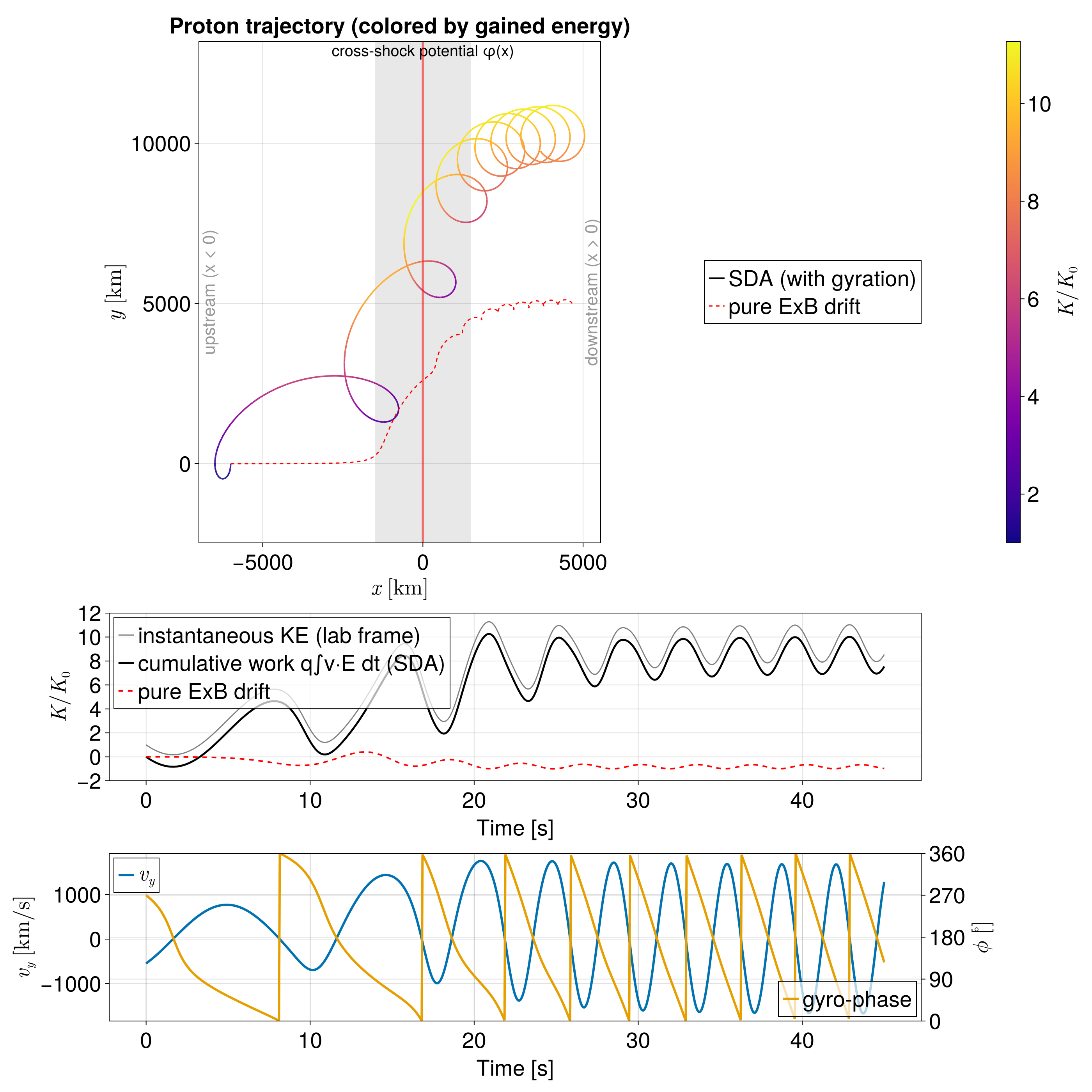

The proton is carried into the red shock front by the normal ExB drift, reflected by the cross-shock potential, and meets the front repeatedly. Each encounter adds energy from $\mathbf{E}$ (the black curve — the cumulative work — climbs with every crossing), so the proton surfs along $+y$ and leaves with a large, sustained gain: shock drift acceleration enabled by the cross-shock potential.